Model Uncertainty in CNNs

Written by Peter Li

Industry is becoming increasingly more reliant on computer vision, with large numbers of diverse applications like robotic surgery and autonomous vehicles. Convolutional neural networks (CNNs) are the typical architecture that underpins such systems. Safety critical applications are now serious candidates for automation despite the significant challenges these problems present. However, there are valid concerns that we are applying black-box algorithms (CNNs) to provide solutions to problems that could result in catastrophic failure. Typically, CNNs provide a mapping from a visual input to an output. In a self-driving car, this output could be the location of a pedestrian on the road. The last thing that an autonomous vehicle manufacturer would want would be an over-confident neural network making incorrect predictions based on an underspecified model. There are many ways to convey the confidence of the model given a prediction, however the most principled way is to use a Bayesian neural network.

Bayesian Neural Networks

A neural network takes an input and outputs something useful. In the case of image classification, the input is an image we wish to classify, and the output would be a probability distribution that represents the chance that the image belongs to each category. The problem with neural networks that work in this way is that they can easily become overconfident in situations that they are not familiar with. This can be attributed to many causes such as a lack of diversity of training data, however it is a particularly tough problem to solve. Indeed recent work suggests that seemingly unimportant changes to a model like a different random parameter initialisation can severely reduce the ability of the model to generalise to unseen data.

A Bayesian neural network represents each prediction as a probability distribution, rather than a single point (in fact the model itself is also a distribution). If we wish to use such a network for inference then we need to sample from this distribution, which means that if we take the same input and perform inference multiple times then each prediction may take a different value. If we take enough samples then the mean of the predictions should represent the equivalent of a classical neural network prediction.

For example, let’s say that we have a classical CNN, and a Bayesian CNN that can both classify cats and dogs and we feed them this image:

A dog that looks like a cat… arguably. (Picture: Gấu Mèo Bắc Mỹ **)

Unfortunately, this dog looks quite a bit like a cat, so our network may predict something like cat: 0.3, dog: 0.7. The classical CNN needs one pass to get its prediction, whereas an equivalent Bayesian network will give us differing predictions, sampled from a distribution. To characterise the distribution accurately we need to take multiple predictions from the Bayesian network:

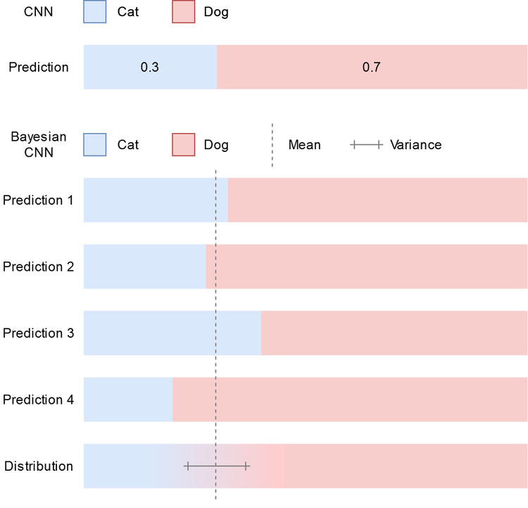
Top: CNN prediction on the input image. Bottom: Sequential Bayesian CNN predictions on the same input, and the inferred distribution

As can be seen in the above image, despite the mean being the same in the classical CNN and the Bayesian one, their individual predictions are not the same. In fact, no prediction sampled from the Bayesian network was ever the same as the classical prediction. Strangely however, they have both predicted the same thing (taking the mean from the Bayesian network as its prediction), but more information is encoded in the output of the Bayesian network.

Take for example the following outputs from two different Bayesian CNNs on the same input image:

Once again, the mean is the same, but the variance is very different. This means that when we sampled the second network, there was a large difference between each prediction, whereas the first network was consistent in predicting numbers close to cat: 0.3, dog: 0.7. Bayesian uncertainty measures allow us to characterise the model uncertainty directly from this variation:

Model Prediction = Mean of the sampled prediction distribution.

Model Uncertainty = Variance of the sampled prediction distribution.

Using this formulation, it is clear that the first network has less intrinsic model uncertainty than the second

How to implement Bayesian Neural Networks

I will not go into the derivations and specifics of Bayes’ theorem and variational inference because there are many great articles that explain this already. What I will present however, is a practical guide to implement these methods in both CNNs, and fully connected neural networks (and therefore almost any model based on matrix-vector multiplication).

The traditional way to infuse Bayesian metrics into neural networks was to change the way we describe the network weights. Instead of each weight being a single value, in a Bayesian network each weight is represented by a distribution, e.g. a Gaussian distribution characterised by a mean and a variance. This method fits nicely with the underlying mathematical description, however, it can be tough to implement and accelerate with modern deep learning libraries. We would have to, for instance, derive gradients for the mean and variance of each weight in the backpropagation step. We would also, at runtime, have to draw sample networks from our weight distributions which could be annoying (given that typically we have to transfer the model parameters to a GPU).

Recent work however has shown that there is a simpler way to achieve our goal of parameterising our weights as a distribution. If we apply dropout to densely connected layers in a neural network then we are essentially applying a Bernoulli distribution over the weights, which has been shown to be exactly what we want to do. Conveniently, also, it is a good way of adding regularisation to our networks, increasing their ability to generalise. Dropout is normally just used in the training stage of our model and removed when we use the trained model for inference, however with a Bayesian network, we want to retain the dropout when we infer. This will give us the behaviour that we need, each time we infer the network on a given sample, it will likely return a slightly different result. The variance of these predictions gives us a principled way of estimating the model uncertainty.

Bayesian Dense Layers

To convert a densely connected layer to a Bayesian dense layer, we can use the following simple PyTorch code as a dropout layer that is called on the output of a PyTorch ‘linear’ layer:

[code here]

This code will function in the same way as the PyTorch dropout layer, however it will maintain its neuron dropping at inference time, optionally the user can provide a dropout mask at runtime which can be used for explicitly controlling which neurons are dropped.

Bayesian Convolution Layers

[code here]

Optical Bayesian CNNs

At Optalysys, we have developed an optical processor that is able to compute convolution operations faster and more efficiently than any electronic processor. The prototype device that we have created in the lab has been tested from a Bayesian perspective, to see if there were any intrinsic differences between model uncertainty for the optical model vs. the equivalent electronic model on the same dataset. This is of particular interest to us because we envisage a future where autonomous vehicles will use optical processors to perceive the world around them. As optical processors are much more efficient than their electronic rivals, this presents a very advantageous use case for devices that are powered by batteries like self-driving cars and drones.

Experiments were carried out on a 2-layer CNN on the MNIST dataset using code similar to the above, modified to run the convolutions on the optical device. Here are the results:

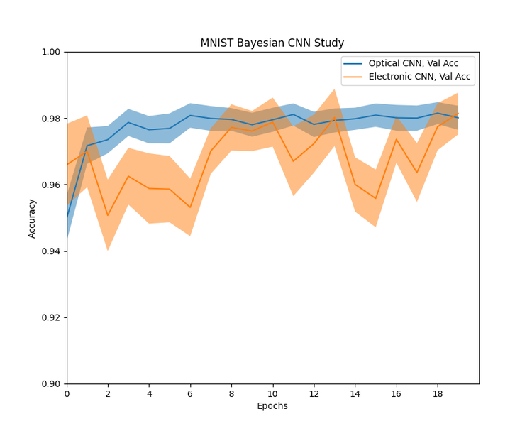
Comparison of an optical and an electronic Bayesian CNN on the MNIST dataset, shaded regions indicate model uncertainty and the central lines are the model accuracies.

We can see that there is still a large amount of excess information even after filtering, so a CNN network often features As can be seen from the initial study, the Bayesian network processed optically seems to behave more consistently, and with a lower model uncertainty than the electronic equivalent. This is a very encouraging result, as it shows that optical neural networks may be ideal for safety critical applications as they are less uncertain than their electronic counterparts. More work needs to be done to understand why this behaviour has emerged, though we do have a few ideas why this may have occurred.

Watch this space.