Experiment with FHE acceleration in our new innovation Lab

Deep learning and fluid dynamics:

AI super resolution using an optical computer
Written by Florent Michel, Joseph Wilson

Table of Contents

In this article, we will discuss super resolution, an AI technique that uses deep neural networks to increase the resolution of images and videos.

At last this scene makes sense. Source

Gone are the days when the above would cause all but the most open-minded to scoff uncontrollably. Today, we really can enhance and upscale low resolution data using the power of deep learning.

Yet even more futuristically, Fourier-optical computing can be used to accelerate this AI processing by reducing the quadratic computational complexity of convolution operations from O(n²) to linear: O(n) (where n is the input size).

What is Super Resoluion?

Simply put, super resolution makes graphics better. Super resolution neural networks are able to take low resolution images (or frames of low resolution video) and output high resolution data that looks good. Better than bilinear or bicubic interpolation. Better to the human eye.

This almost seems like magic, and for good reason: somehow these networks are able to take grainy, pixelated inputs and transform them into high resolution, great looking images.

All this can be achieved without explicitly using any of the traditional computer graphics techniques such as anti-aliasing, smoothing and interpolation. What we are seeing with super resolution is the magic of deep learning based computer vision (CV). Neural networks are able to infer what a pixelated image depicts by using prior knowledge and patterns learned from examples.

How Super Resolution Works

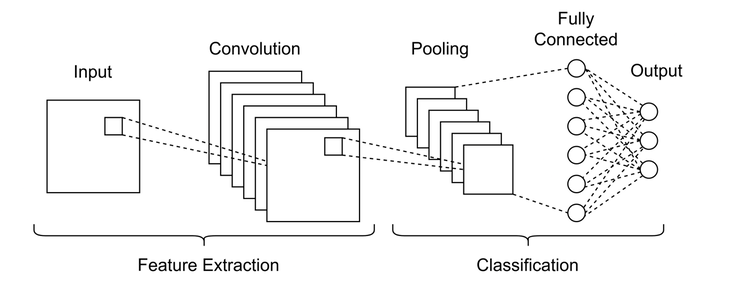
AI Super resolution usually leverages deep neural networks optimised for CV. Convolutional neural networks (CNNs) have been a mainstay of CV for several decades, and are normally used for things like image classification, an early example of which is how Yann LeCun used CNNs to learn how to classify handwritten digits, allowing cheques to be cashed autonomously.

Background: CNNs for classification

Classification CNNs typically have a structure like this:

Image of a typical CNN used for classification. Larger images are pooled down to smaller images sequentially, eventually the smaller images connect to a dense layer for classification.

Typically, images are fed into the network and convolved with many filters, the filtered images are combined to make up the output of a ‘multichannel convolution’ layer. The layer output is usually the same size as the input.

Subsequent convolution layer outputs are often reduced in size via operations such as max-pooling. Once the data has been pooled to a reasonable size (sometimes as small as a single pixel), it can be fed into dense or fully-connected layers for classification.

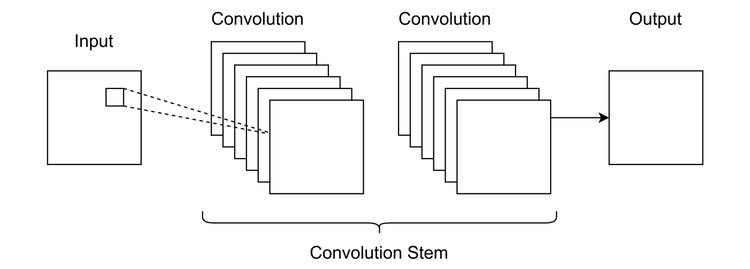
Background: CNNs for other systems

More modern CNN applications include autonomous driving, robotic surgery and medical screening (these applications go beyond image classification, into systems control and semantic segmentation). Apps like Faceswap are a good example of contemporary CV, where both the CNN input(s) and output(s) are images. Such systems are able to manipulate a pair of images, non-invasively transplanting the face of one onto the head of another.

A Faceswap-esque CNN may have a structure like this:

In an image->image CNN, dimensionality of the input is not necessarily reduced. Sequential convolution layers can be used without pooling.

Or like this:

Typical U-Net style CNN, where the intermediate layer outputs are reduced in size, before being sequentially upsampled to an increased size. The reduction in size is usually accompanied by an increase in the channel dimension to stop too much information being thrown away in the middle.

CNNs for super resolution

In a similar way, super resolution networks take an image and output another. The only difference from the above architectures is that the input image and output image are not the same size. Rather the output should be of a higher resolution, while still faithfully depicting the original scene.

If we desire the output of the CNN to be of a higher resolution than the input, then we require some form of non-standard CNN layer, something which is the opposite of a typical convolution ⇨ pool block in a classification CNN. This is known as an upsampling layer.


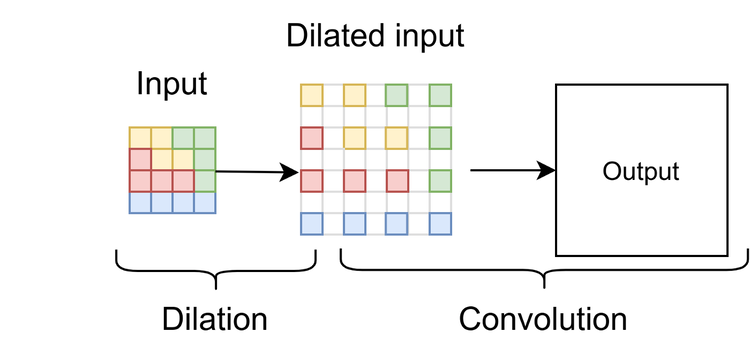
Dilation upsampling (aka sup-pixel convolution),

One technique used is to dilate the input image, effectively making a sparse matrix from the original that is double the size in height and width. This sparse matrix is used as the input to a standard convolution layer. Dilation upsampling is a simple and natural solution to achieve super resolution. The downside of this method is that the CNN filters will always cover regions of zero valued pixels, effectively wasting computation.

Image size can be increased by convolving with a dilated image, unfortunately it involves wasted computation as the filter sees many zero-valued elements in the dilated image.


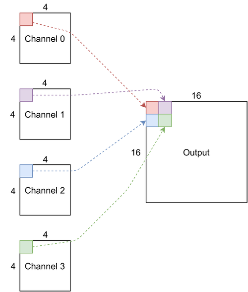
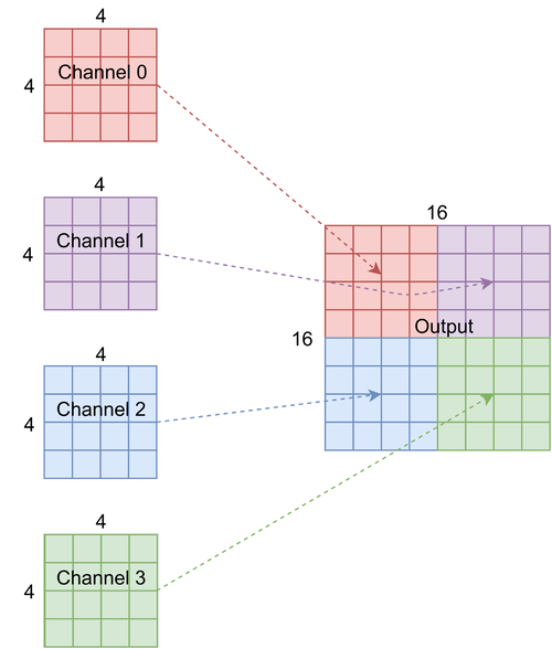
Multi-channel reshape upsampling (aka resize convolution)

Channel upsampling takes a multi-channel image (such as the output from a convolution layer) and reshapes the data into fewer channels but with larger height and width.

In a classification CNN, there are usually sequential pooling layers, designed to reduce the size of the internal data representation and thereby the computational complexity. In order to make sure unrecoverable information is not being destroyed, convolution layers or blocks typically increase the channel count. For instance a 32-channel 16×16 input may be converted into a 64-channel 8×8 output.

Upsampling requires the opposite to take place. Image resolution should increase, therefore it is sensible to also reduce the channel count. This can be achieved by reshaping. For example, a 16-channel 100×100 input could be reshaped into a 4-channel 200×200 output. Compared to the dilated convolution, this is just as expressive of a solution (with the same network parameter count), without the compute penalty.

One way to think of this is to take the top-left pixel of the first 4 output channels, which when arranged into 2×2 grid will make up the top left 2×2 quadrant of a single output channel. Then this can be repeated for all pixel locations and channels ad absurdum.

How multiple channels can be combined to create a larger single channel of larger resolution. In this example 4 input channels of size 4×4 are upsampled into a single 16×16 output channel.

We could of course just reshape the output tensor naively, however this might cause problems, because CNNs preserve the spatial information of their inputs, so it makes sense to keep pixels in the same spatial location together.

This image shows a more naive approach to reshape upsampling. The problem here is that the global spatial information in each of the input channels is incorrectly combined into a local spatial location.


When to upsample

One final consideration is when the upsampling should take place. There is no ‘correct’ solution, just a few different ideas with varying results.

  • Upsample in the final layer. This is the most simple idea; however, the authors of Deep Learning for Image Super-resolution: A Survey note that for larger upsample factors such as x8, this method is not the best.

  • Upsample gradually throughout the network, similar to the sequential pooling throughout classification CNNs.

  • Upsample and down-sample throughout the network, e.g. a U-Net architecture.


PyTorch implementation of super resolution

Data & hardware

Data for super resolution experiments is abundant. Images need not be classified or labelled in any way, the only prerequisite is that training images should be at least as big as the resolution we wish to upsample to.

We used a python web scraper that downloads images returned by Google image search when fed keywords like ‘lion’:

from selenium import webdriver
from PIL import Image
import os
import time
import io
import requests
import hashlib

def fetch_image_urls(query: str, max_links_to_fetch: int, wd: webdriver, sleep_between_interactions: int = 1):
    def scroll_to_end(wd):
        wd.execute_script("window.scrollTo(0, document.body.scrollHeight);")
        time.sleep(sleep_between_interactions)

    search_url = "https://www.google.com/search?safe=off&site=&tbm=isch&source=hp&q={q}&oq={q}&gs_l=img"
    wd.get(search_url.format(q=query))
    image_urls = set()
    image_count = 0
    results_start = 0
    load_mode_iterations = 0

    while image_count < max_links_to_fetch:
        scroll_to_end(wd)
        thumbnail_results = wd.find_elements_by_css_selector("img.Q4LuWd")
        number_results = len(thumbnail_results)
        print(
            f"Found: {number_results} search results. Extracting links from {results_start}:{number_results}")
        for img in thumbnail_results[results_start:number_results]:
            try:
                img.click()
                time.sleep(sleep_between_interactions)
            except Exception:
                continue
            actual_images = wd.find_elements_by_css_selector('img.n3VNCb')
            for actual_image in actual_images:
                if actual_image.get_attribute('src') and 'http' in actual_image.get_attribute('src'):
                    image_urls.add(actual_image.get_attribute('src'))

            image_count = len(image_urls)
            if (len(image_urls) >= max_links_to_fetch):
                print(f"Found: {len(image_urls)} image links, done!")
                break
        else:
            print("Found:", len(image_urls),
                  "image links, looking for more ...")
            time.sleep(1)
            load_mode_iterations += 1
            if load_mode_iterations > 15:
                print(
                    f"Giving up. Found: {len(image_urls)} image links, done!")
                return image_urls
            load_more_button = wd.find_element_by_css_selector(".mye4qd")
            if load_more_button:
                wd.execute_script("document.querySelector('.mye4qd').click();")
        results_start = len(thumbnail_results)
    return image_urls


def persist_image(folder_path: str, url: str):
    try:
        image_content = requests.get(url, timeout=10).content
    except Exception as e:
        print(f"ERROR - Could not download {url} - {e}")
    try:
        image_file = io.BytesIO(image_content)
        image = Image.open(image_file).convert('RGB')
        _w, _h = image.size
        min_dim = min(_w, _h)
        if (min_dim < IMAGE_SIZE):
            raise RuntimeError('Image too small: ' + str(_w) + ' ' + str(_h))
        else:
            half_min_dim = int(min_dim / 2)
            centre_h = int(_h / 2)
            centre_w = int(_w / 2)
            start_h = centre_h - half_min_dim
            start_w = centre_w - half_min_dim
            end_h = start_h + min_dim
            end_w = start_w + min_dim
            image = image.crop((start_w, start_h, end_w, end_h))
            image = image.resize((IMAGE_SIZE, IMAGE_SIZE))

        file_path = os.path.join(folder_path, hashlib.sha1(
            image_content).hexdigest()[:10] + '.jpg')
        with open(file_path, 'wb') as f:
            image.save(f, "JPEG")
        print(f"SUCCESS - Saved image from {url}")
    except Exception as e:
        print(f"ERROR - Could not save {url} - {e}")


def search_and_download(search_term: str, driver_path: str, target_path='images', number_images=5):
    target_folder = os.path.join(target_path, "_".join(search_term.split()))
    if not os.path.exists(target_folder):
        os.makedirs(target_folder)
    with webdriver.Chrome(executable_path=driver_path) as wd:
        res = fetch_image_urls(search_term, number_images,
                               wd=wd, sleep_between_interactions=0.1)
    for elem in res:
        persist_image(target_folder, elem)


DRIVER_PATH = 'scraping/chromedriver.exe'
IMAGE_SIZE = 256

if __name__ == '__main__':
    search_and_download('citrus fruit', DRIVER_PATH, number_images=1000)
    search_and_download('leaves', DRIVER_PATH, number_images=1000)
    search_and_download('rainforest', DRIVER_PATH, number_images=1000)
    search_and_download('cuttlefish', DRIVER_PATH, number_images=1000)
    search_and_download('lion', DRIVER_PATH, number_images=1000)

Images large enough were downloaded, cropped square and resized to our target upscaled resolution: 256². This process was repeated until we had a unique dataset of around 14,000 images. The images were split into 70% training and 30% validation subsets. PyTorch dataloaders were used to load the datasets.

Training setup

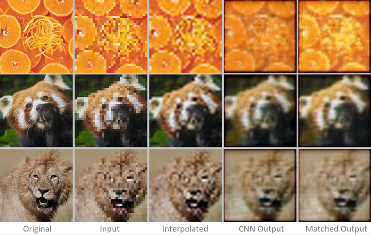
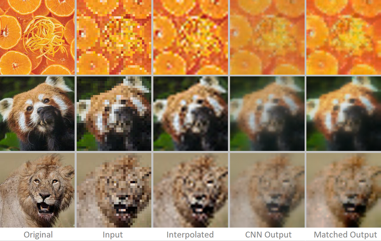
During training and validation, the 3-channel, 256²-sized images in the dataset were used as the ground truth values. Inputs to the network were created by downsizing the ground truth images to 3-channel 32² using the nearest neighbour algorithm. Electronic training took place on an Nvidia Quadro P6000.

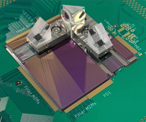
We wanted our convolutional layers to be performed by Optalysys’ optical chip, so we used our PyTorch layer to interface with the Optalysys silicon photonic free-space Fourier optical chip in the lab. Prototype networks were run electronically, once suitable hyperparameters were chosen, the optical network could be called by passing ‘optical=True’ to our model when initialising.


Our upsampling technique

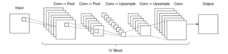
We wrote code that defines an upsample block of varying channel depth and convolutional layer count. The block could then be parameterised into an entire network with a single upsample at the end, or multiple blocks could be stacked together to create larger end-to-end network upsample factors. The block can also be combined with conv → pool type blocks for a U-net super resolution architecture.


Avoiding checkerboarding

Upsampling generally can suffer from ‘checkerboarding’, clearly visible in the image below:

Example of checkerboarding. Original Image Source

This paper discusses it in depth, and provides a principled method to avoid it. As we used the so called ‘resize convolution’ upsampling method, the prescribed fix to checkerboarding is to initialise the weights and biases of the convolutional kernels which contribute to the same output quadrant to the same value.

Padding

A further generic issue with upsampling CNNs can occur at the border of the output image. Generally in CNNs, padding is used to keep the height and width of layer inputs and outputs consistent. Zero padding is the traditional choice, however this effectively would mean that we were surrounding each image with black border, which would lead to visual artefacts in the upscaled image. For this reason we used ‘replicate’ type padding so that the border would be made up of sensible values.


Upsample block PyTorch code

import torch
import torch.nn as nn
import torch.nn.functional as F
from pytorchlayer.opt_conv_layer import OptConvLayer

# makes a matrix sparse by padding within: e.g. [1,2,3] -> [0,1,0,2,0,3,0]
def pad_within(x, stride=2):
    w = x.new_zeros(stride, stride)
    w[0, 0] = 1
    return F.conv_transpose2d(x, w.expand(x.size(1), 1, stride, stride), stride=stride, groups=x.size(1))

# takes a 4d array (BxCxHxW) where (channels // 4) == 0
# returns a channel upsampled array with H and W x2 and C /4
def channel_upsample2d(x):
    start_shape = x.shape
    target_shape = (start_shape[0], int(start_shape[1] / 4), start_shape[2]*2, start_shape[3]*2)
    assert(x.ndim == 4)
    assert(not (x.shape[1] % 4))
    x = pad_within(x, 2)
    w = x.view(-1, 4, x.shape[2], x.shape[3])
    w[:, 1] = w[:, 1].roll(shifts=(1,0), dims=(1,2))
    w[:, 2] = w[:, 2].roll(shifts=(0,1), dims=(1,2))
    w[:, 3] = w[:, 3].roll(shifts=(1,1), dims=(1,2))
    w = w.sum(axis=1)
    return w.view(target_shape)

# convolutional block that takes a 4d input (BxCxHxW), does multi channel-convolutions, internally increases the channel
# dimension to 4x the input channel dimension, then multichannel upsamples to output something with H & W 2x increased 
class UpsampleBlock(nn.Module):
    def __init__(self, depth, length, kernel_size, padding, optical=False, padding_mode='zeros') -> None:
        super(UpsampleBlock, self).__init__()
        self.conv_layer_count = length
        self.depth = depth
        
        if optical:
            self.conv_layers = nn.ModuleList([
                OptConvLayer(depth if ch == 0 else depth * 4, depth * 4, kernel_size=kernel_size, padding=padding,
                             perfect_gradient=True)
                for ch in range(self.conv_layer_count)])
        else:
            self.conv_layers = nn.ModuleList([
                nn.Conv2d(depth if ch == 0 else depth * 4, depth * 4, kernel_size=kernel_size, padding=padding,
                          padding_mode=padding_mode)
                for ch in range(self.conv_layer_count)])

        self.fix_initialisation()

    def forward(self, x):
        layer_input = x
        for i, layer in enumerate(self.conv_layers):
            x = F.elu(layer(x))
        # add residual connections
        ind = torch.tensor([i for i in range(0, self.depth*4, 4)])
        for i in range(4):
            x[:, ind+i] += layer_input
        return channel_upsample2d(x)

    # fix checkerboard pattern
    def fix_initialisation(self):
        with torch.no_grad():
            for q in range(self.conv_layers[self.conv_layer_count-1].weight.shape[0] // 4):
                for ich in range(self.conv_layers[self.conv_layer_count-1].weight.shape[1]):
                    w0 = self.conv_layers[self.conv_layer_count-1].weight[q * 4, ich]
                    b0 = self.conv_layers[self.conv_layer_count-1].bias[q * 4]
                    for i in range(4):
                        self.conv_layers[self.conv_layer_count-1].weight[q * 4 + i, ich] = nn.Parameter(w0)
                        self.conv_layers[self.conv_layer_count - 1].bias[q * 4 + i] = nn.Parameter(b0)

For our experiment we used 3 upsample blocks of depth 4 and length (number of internal multichannel convolution layers) 4, 2 and 1 from input to output respectively. We defined an end-to-end model consisting of a single convolution layer with 3×3-sized filters, several unsample blocks with 3×3-sized filters, then a 1×1 convolution layer at the end for channel reduction.

Here’s the code for the model:

import torch.nn as nn
import torch.nn.functional as F
from upsample import UpsampleBlock
from pytorchlayer.opt_conv_layer import OptConvLayer


class SuperResolutionModel(nn.Module):
    in_channels = 3
    out_channels = 3
    upsample_block_depth = [4, 4, 4]
    upsample_block_length = [4, 2, 1]
    upsample_block_count = 3
    upsample_kernel_size = 3
    default_padding = 1

    def __init__(self, optical=False):
        super(SuperResolutionModel, self).__init__()
        if optical:
            self.c1 = OptConvLayer(self.in_channels, self.upsample_block_depth[0], kernel_size=self.upsample_kernel_size,
                                   padding=self.default_padding, perfect_gradient=True)

            self.cf = OptConvLayer(self.upsample_block_depth[-1], self.out_channels, kernel_size=1,
                                   padding=0, perfect_gradient=True)

        else:
            self.c1 = nn.Conv2d(self.in_channels, self.upsample_block_depth[0], kernel_size=self.upsample_kernel_size,
                                padding=self.default_padding, padding_mode='replicate')

            self.cf = nn.Conv2d(self.upsample_block_depth[-1], self.out_channels, kernel_size=1,
                                   padding=0, padding_mode='replicate')

        self.c_stem = nn.ModuleList([
            UpsampleBlock(
                self.upsample_block_depth[i], self.upsample_block_length[i], self.upsample_kernel_size,
                self.default_padding, optical=optical, padding_mode='replicate')
            for i in range(self.upsample_block_count)])

    def forward(self, x):
        x = F.elu(self.c1(x))
        for block in self.c_stem:
            x = block(x)
        x = self.cf(x)
        return x

For training, we found that a batch size of 4 worked well for our experiments. We trained the model with a stepped learning rate starting at 0.01 with a gamma of 0.8 for around 15 epochs.


Choice of loss function — 1) Pixel loss mean squared error

Initially we tried a simple mean squared error (MSE) loss term taken using the network output and the original 256² image, this worked fairly well, but the results were not great:

Left: Original image (256²), Centre-left: Downsampled image (32²), Centre: Bicubic interpolation of downsampled image (256²), Centre-right: CNN output trained with MSE loss (256²), Right: CNN output trained with MSE loss (256²) + histogram matching with original image. Top Image, Middle Image, Bottom Image

The CNN output is arguably nicer to look at than the interpolated image, with less pixel artefacts, however it is not fantastic. Problems with the CNN image include blurring and slight colour issues. Histogram matching was used to attempt to recover the lost colour which was somewhat successful.

The above images are a good example of the general efficacy of the neural network super resolution across the validation set. These results are decent, but what can be done to improve them? Perhaps a different loss function…

2) Mean gradient error

Mean gradient error (MGE) has been suggested as a method to reduce the blurriness of the CNN output, the idea is to use a horizontal and vertical edge filter on the prediction and the target image, taking the MSE between the two pairs of filtered images. This loss term should heavily penalise networks that make blurry predictions, thus sharpening the output.

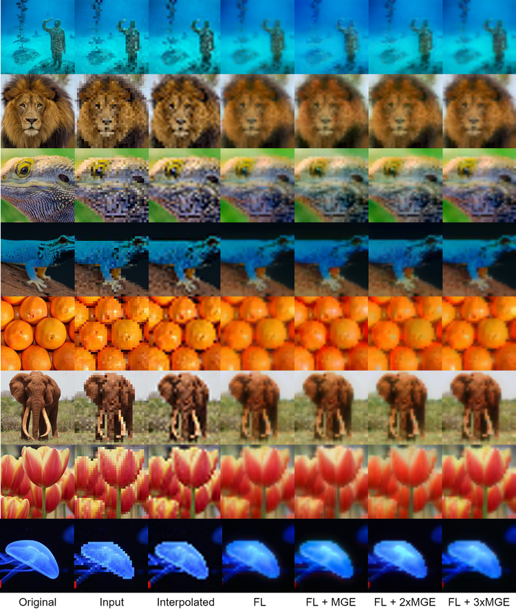
def mge_loss(prediction, target):
    x_filter = torch.tensor([[-1, -2, -1],
                              [0,  0,  0],
                              [1,  2,  1.0]]).unsqueeze(0).repeat(3, 1, 1).unsqueeze(0).cuda() / 8
    y_filter = torch.tensor([[-1, 0, 1],
                              [-2, 0, 2],
                              [1,  0, 1.0]]).unsqueeze(0).repeat(3, 1, 1).unsqueeze(0).cuda() / 8

    replication_pad = nn.ReplicationPad2d(1)
    gx_prediction = F.conv2d(replication_pad(prediction), x_filter)
    gy_prediction = F.conv2d(replication_pad(prediction), y_filter)
    gx_target = F.conv2d(replication_pad(target), x_filter)
    gy_target = F.conv2d(replication_pad(target), y_filter)
    mge_x = F.mse_loss(gx_prediction, gx_target) / 2.0
    mge_y = F.mse_loss(gy_prediction, gy_target) / 2.0
    return (mge_x + mge_y) * mge_loss_scale

Here are the same images, inferred by a network trained with a combined loss term of MSE + MGE, where the scale of the MSE term and MGE term were both set to 1.

Left: Original image (256²), Centre-left: Downsampled image (32²), Centre: Bicubic interpolation of downsampled image (256²), Centre-right: CNN output trained with MSE + MGE loss (256²), Right: CNN output trained with MSE + MGE loss (256²) + histogram matching with original image.

These outputs do look better in some ways, they are somewhat sharper than the MSE network outputs, though the difference is not stark. There has also emerged a new problem at the image border. Is this network any better than MSE? This is of course difficult to quantify. It seems though, like the CNN outputs are a fairly realistic attempt to render the scene, if it was being viewed slightly out of focus. Arguably these outputs look more ‘realistic’ than the interpolated images and could be useful for certain applications.

Various combinations of MSE and MGE loss terms were tried with different weightings, however the results were still not fantastic. MGE in theory should lead to crisper outputs but in reality the results are still quite unfocused.

3) Feature loss

The problem, it seems, with an intuitive pixel based loss function is that it leads mediocre results. What we really would like to use is a loss function similar to human perception, i.e. if the images look similar to the original full size image, then this is good, even if there are many pixels which are individually inaccurate.

Johnson et al. outline ideas to achieve perceptual loss functions used in their work for super resolution and style transfer. The idea is simple:

  • Take a pre-trained CNN like VGG-16 trained on the ImageNet dataset.

  • Pass the pre-trained model the ground truth image and the super resolution CNN output.

  • Take an output tensor from a feature-extracting layer in the pre-trained VGG model for both inputs.

  • Use the normalised, squared Euclidian distance between the two feature tensors as the loss term.

  • When backpropagating, freeze the weights of the pre-trained VGG model.

Here is a code snippet that shows how this works, taking the output from the VGG-16 layer relu2_2:

def normalised_squared_euclidean_distance(m_1, m_2):
    return torch.mean(torch.square(m_1 - m_2))

def vgg_feature_loss(prediction, target, loss_model):
    p_features = loss_model.forward_features(prediction).relu2_2
    t_features = loss_model.forward_features(target).relu2_2
    return normalised_squared_euclidean_distance(p_features, t_features)

The above code requires a loss_model object, which can be instantiated from a class such as this (the example also has style loss functionality as mentioned by Johnson et al., though style loss is not recommended for super resolution):

def normalised_squared_euclidean_distance(m_1, m_2):
    return torch.mean(torch.square(m_1 - m_2))

def vgg_feature_loss(prediction, target, loss_model):
    p_features = loss_model.forward_features(prediction).relu2_2
    t_features = loss_model.forward_features(target).relu2_2
    return normalised_squared_euclidean_distance(p_features, t_features)

What this loss function is evaluating is: does the generated image look like the original? Does a network like VGG-16 trained on ImageNet see the same features in the image that are relevant to the image contents as defined by the ImageNet image class? This might seem like a rather foolhardy question given that the images in our dataset do not necessarily contain the same subject matter as ImageNet, however this is not a problem.

ImageNet is a very large dataset comprising many different heterogeneous objects. In order to classify them well, a neural network needs to recognise general features such as edges, textures and shapes. As such networks trained on ImageNet have a good general feature extraction ability, so much so that they can be repurposed to work with data outside of the ImageNet dataset’s statistical distribution with minimal training using transfer learning. For this reason, using a pretrained VGG-16 architecture on ImageNet is a sensible choice for a perceptual loss discriminator.

We trained the feature loss network with exactly the same network architecture and hyperparameters, but with the feature loss (FL) loss function, and here are the results:

Left: Original image (256²), Centre-left: Downsampled image (32²), Centre: Bicubic interpolation of downsampled image (256²), Centre-right: CNN output trained with feature loss (256²), Right: CNN output trained with feature loss (256²) + histogram matching with original image.

These images look better than the interpolated ones to us. Unfortunately they still look a little blurry, so we tried adding in a weighted MGE loss term onto the feature loss.


Further comparisons of different loss functions:

We tried out networks with different combinations of FL and MGE terms, weighted as (1, 0), (1, 1), (1, 2) and (1, 3) respectively:

Left: Original image (256²), Second from left: Downsampled image (32²), Third from left: Bicubic interpolation of downsampled image (256²), Centre to Right: Various CNN outputs with different loss terms (256²). Image 1, Image 2, Image 3, Image 4, Image 5, Image 6, Image 7, Image 8

The results from the neural networks are all very similar, however from the FL column onward, we do see a slight increase in the sharpness of the images, which we can explain by the increase influence of the MGE term. We personally liked the FLE + MGE column the most, though it is up for debate.

Super Resolution on an Optical Computer

Background: The Optalysys approach

At Optalysys, we develop optical chips driven by silicon photonics. Our next-generation, high-speed chip will leverage precision free-space optics to perform optical Fourier transform operations at speeds and efficiencies far exceeding the best electronic Fourier transform cores. Currently we have a proof-of-concept thermally driven demonstrator system in the lab.

The thermally driven silicon photonics/free space optics device in the lab.

The Fourier transform can be used (via the convolution theorem) to reduce the computational complexity of the convolution operation from quadratic to linear. Hence if we are able to convert data into its frequency representation, we can infer with- and train CNNs with far fewer operations. This reduction in operations (typically multiply and accumulate or MAC operations) is depicted in the chart below:

Chart depicting the MAC reduction from using Fourier transforms to calculate convolutions in the spectral domain vs general matrix multiply convolution (GEMM) in various CNN architectures. R-34 7×7 is a model with the same structure as R-34 but with 7×7 sized kernels throughout. MACs calculated for batch size of 128.

We also describe this idea in more detail in this article.

Super resolution experiments on an optical computer

Our hardware in the lab is addressable via a PyTorch interface. It was therefore painless to run the super resolution models prototyped above on our optical chips to gauge its performance. We ran the model discussed above optically by passing ‘optical=True’ when instantiating the PyTorch model, and compared it with the electronic version:

Comparison of the optical and electronic CNN. Image 1, Image 2, Image 3, Image 4, Image 5

We see that generally, the performance of the optical CNN is at least as good as the electronic network. In some ways it is better; the colours are more accurate and there are less artefacts when the images are viewed up close.

Close up of the optical CNN (left) and the electronic CNN (right). The colours in the optical CNN output are more faithful to the original and there are less strange artefacts overall.


Going beyond 256²

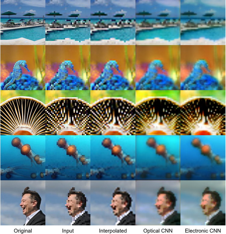
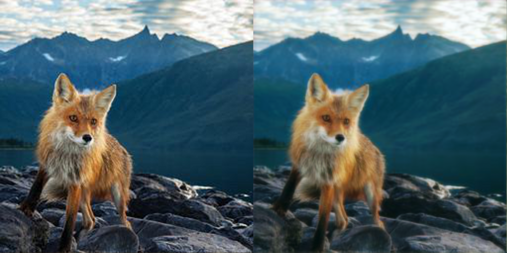
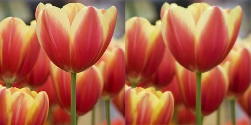
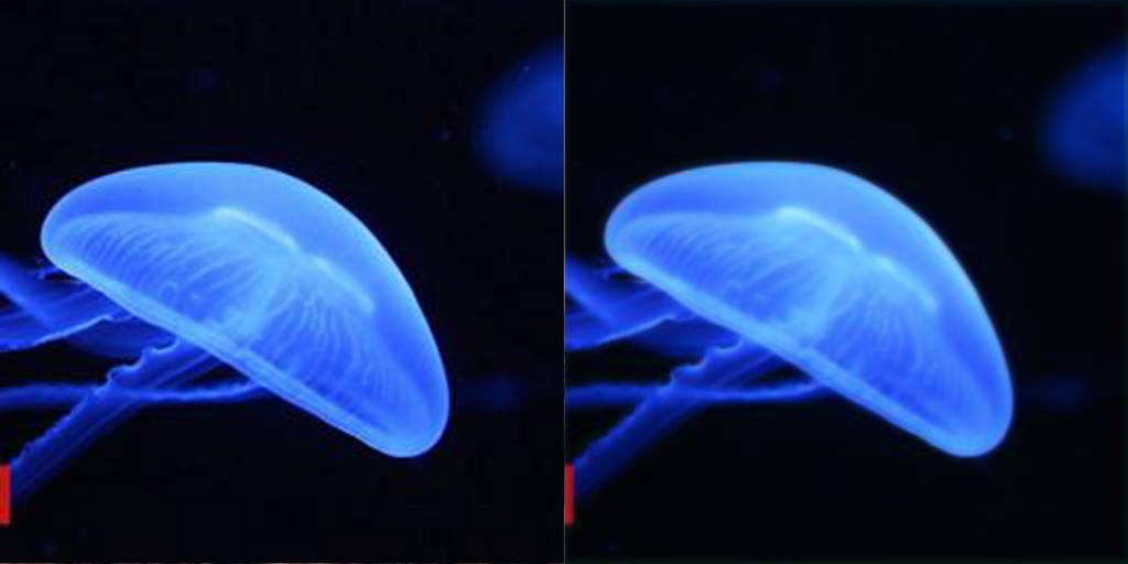
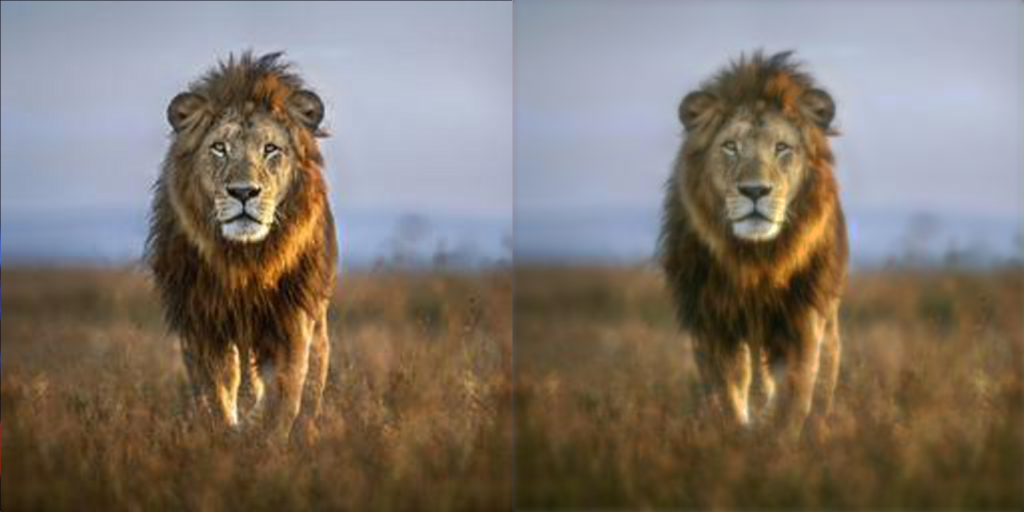
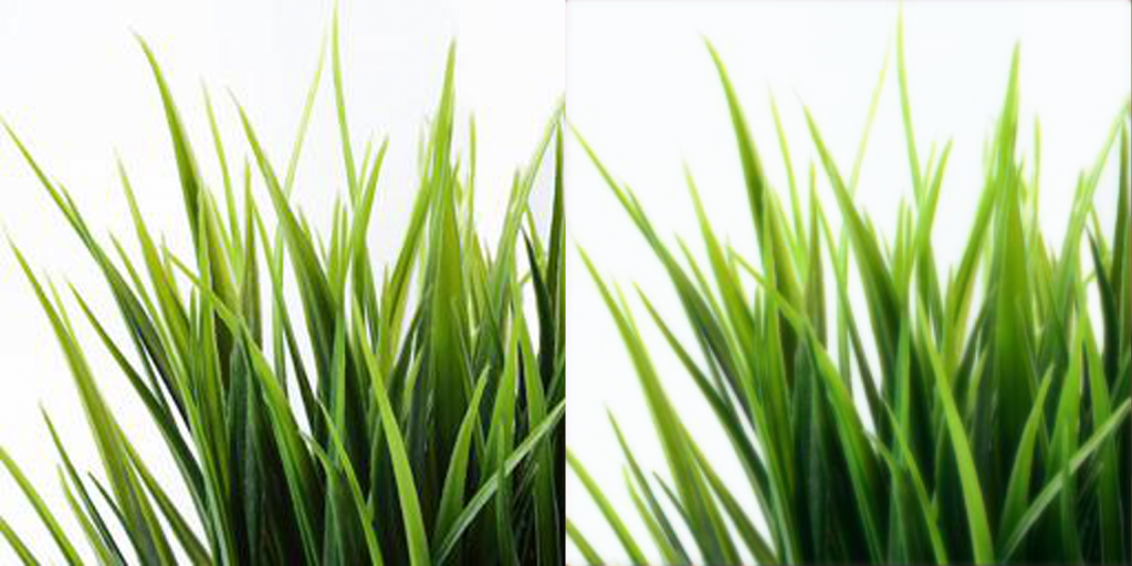
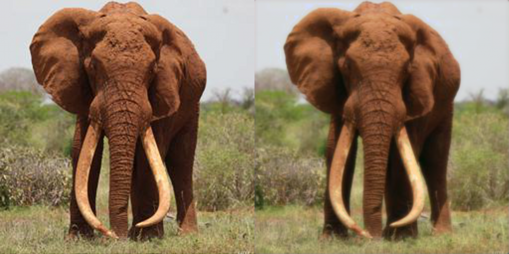
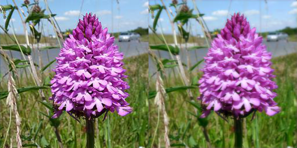
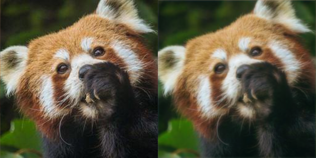
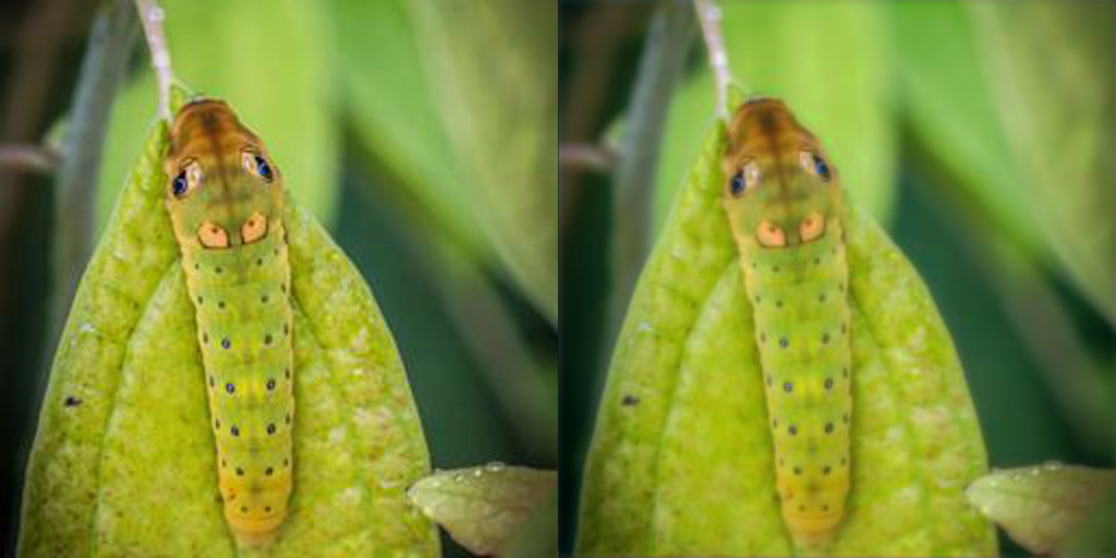
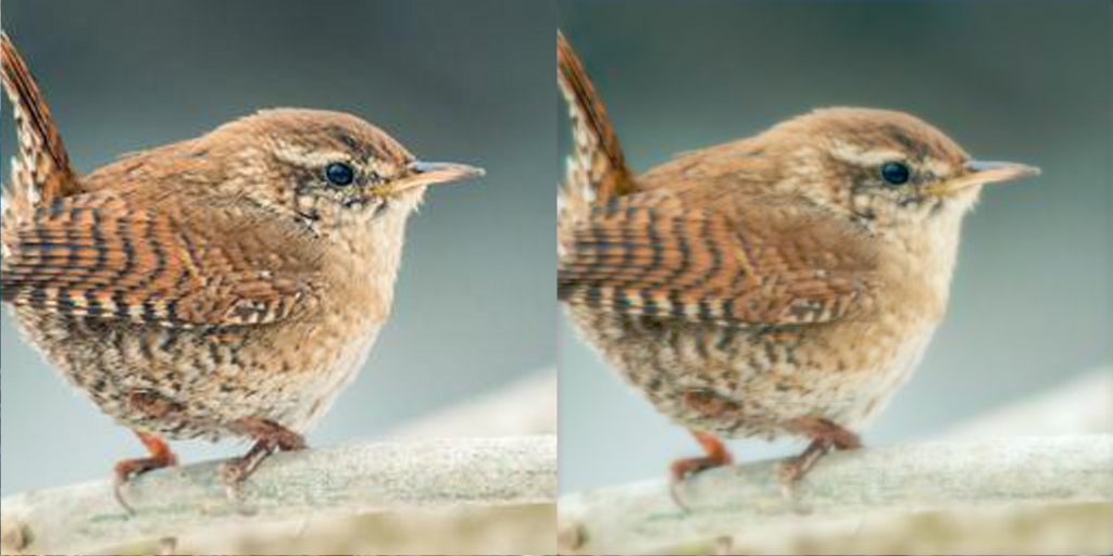
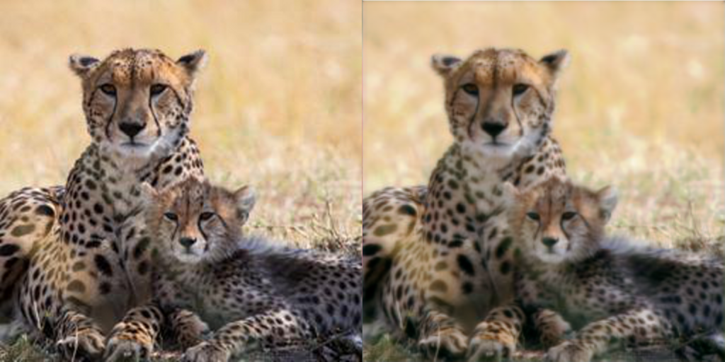
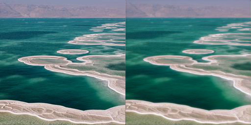
The awesome thing about end-to-end CNN architectures (unlike transformers and CNNs with dense layers) is that they will work for any inputs of any size. The convolutional layers work in the same way, regardless of the height and width of the input. This means that we can use the same network, originally trained on 32² 8x upscaling, on larger inputs. We can, for instance, take the 256² data in the dataset and upscale it to 2048².

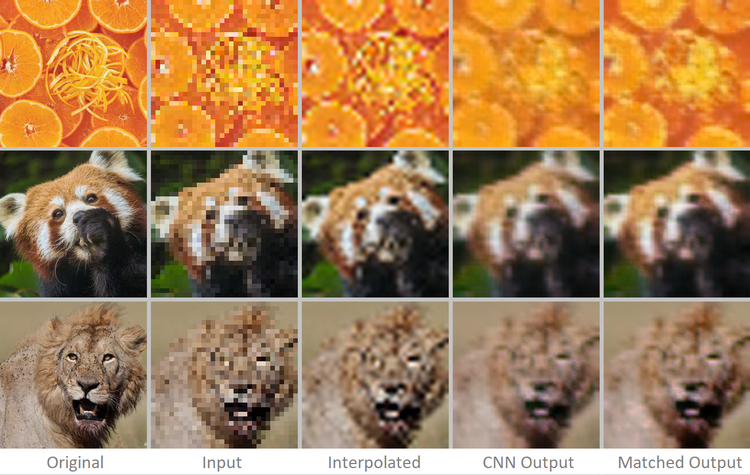
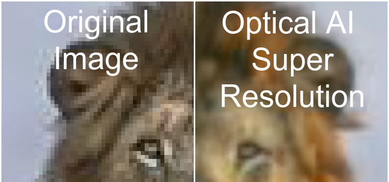
As the data was originally gathered from scraping the web, there are artefacts in many of the images consistent with lossy JPEG like compression. Can the CNN be used to restore the image quality while also increasing the resolution? Below are some examples of the networks being used in this way; we were amazed by the results.

Thanks for reading!

by Ed@Optalysys — [email protected]


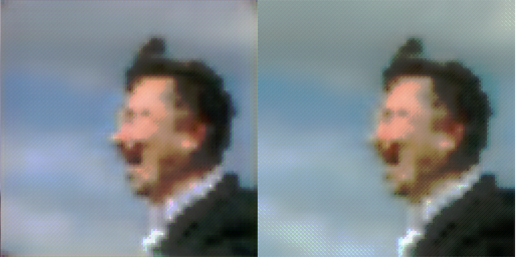
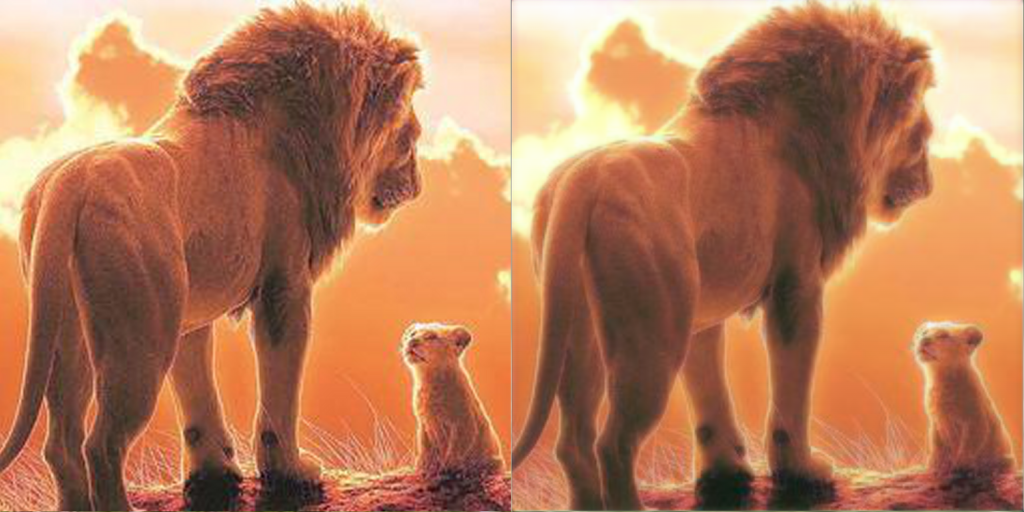
Left: Bicubic upsampling — 256² → 2048²

Original images have some lossy compression artefacts.


Right: Optical CNN — 256² → 2048²

CNN was trained on 32² → 256² x8 upsampling.

Images obtained from Google, used in accordance with fair use. If there are any copyright issues with images, please contact me and I will take them down.

Image Sources:

Thumbnail: Serengeti Lion

  1. Can you enhance that?

  2. Jellyfish

  3. Orange zest

  4. Red panda

  5. Lion

  6. Underwater museum

  7. Lion

  8. Iguana

  9. Electric-blue gecko

  10. Oranges

  11. Elephant

  12. Flowers

  13. Jellyfish

  14. Sun loungers

  15. Seahorse

  16. Mushroom

  17. Elon Musk

  18. The Lion King

  19. Fox

  20. Grass

  21. Road verge flower

  22. Flower

  23. Caterpillar

  24. Wren

  25. Leopards

  26. Beach

Subscribe

Sign up with your email address to receive news and updates from Optalysys.

Please enable JavaScript in your browser to complete this form.
We respect your privacy.