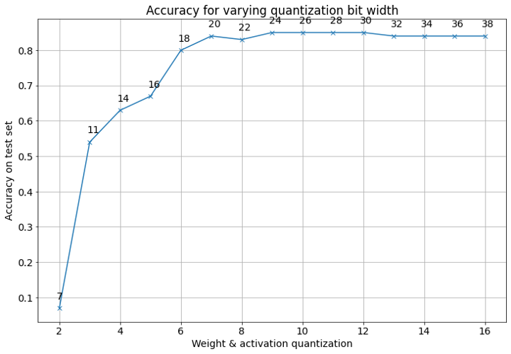
In the PyTorch example, we mentioned how the size of the intermediary values stored in accumulators while the neural network is running inference often greatly exceed that of the inputs. Here we will briefly look at the implications of this on TFHE, and the prospect of running larger deep learning models in TFHE in the future.

We are going to simulate a larger neural network for image classification, trained on the Fashion MNIST dataset, running in TFHE. Due to the size of the images — 728 pixels each — making the input size 728, the model is only capable of running inference in TFHE if 2 bits are used for quantising the inputs. This leads to an expectedly poor accuracy, of only 14%, down from a plaintext accuracy of nearly 90%.

Any larger bit width results in error, as some of the intermediary results end up requiring more than 8 bits to represent — exceeding TFHE’s current limit.
However, using the Virtual Lib tool from Concrete ML, we can simulate running the TFHE circuit in plaintext, with quantisation bit widths that exceeds the current limitations, and obtain results on how the accuracy, as well as how the maximum required accumulator size for storing intermediary values scales with the quantisation bit width.

This is important, as the future development pathway for TFHE incorporates higher bit precision. This tool thus aids understanding in the applications where TFHE will be useful in the future.

Below is the code and the results obtained;

# Importing relevant libraries and modules

import torch
import matplotlib.pyplot as plt
import numpy as np
import pandas as pd
import torch.nn as nn
import torch.nn.functional as F

# Importing the Fashion MNIST Dataset as Pandas dataframes

training = pd.read_csv('fashion-mnist_train.csv')
testing = pd.read_csv('fashion-mnist_test.csv')

# Splitting the dataframes into X (features) and y (targets)

X_train, y_train = training.loc[:, training.columns != 'label'], training.loc[:, training.columns == 'label']
X_test, y_test = testing.loc[:, testing.columns != 'label'], testing.loc[:, testing.columns == 'label']

# Converting dataframes to NumPy arrays

X_train = X_train.to_numpy()
X_test = X_test.to_numpy()
y_train = y_train.to_numpy()
y_test = y_test.to_numpy()

# Normalising the X values by dividing by 255, as each feature is the value of a
# greyscale pixel, which is a number between 0 and 255 inclusive

X_train, X_test = X_train/255, X_test/255

# One Hot encoding the labels, transforming them from integer values (each representing)
# a category of clothing) to One Hot encoded binary arrays

from sklearn.preprocessing import OneHotEncoder

onehot_encoder = OneHotEncoder()
y_train = onehot_encoder.fit_transform(y_train).toarray()
y_test = onehot_encoder.fit_transform(y_test).toarray()

# Define a simple fully connected neural network using PyTorch
# It has a single hidden layer with 128 neurones, and an outpt layer of 10 neurones
# corresponding to the 10 different output classes

class FCNN(nn.Module):
    def __init__(self, input_size):
        super().__init__()
        self.linear1 = nn.Linear(input_size, 128)
        self.linear2 = nn.Linear(128, 10)
        self.relu = nn.ReLU()
    
    def forward(self, x):
        x = self.linear1(x)
        x = self.relu(x)
        x = self.linear2(x)
        return x

# Initialising the model with 728 input neurones; defining the optimiser
# and the loss functions

model = FCNN(X_train.shape[1])
learning_rate = 0.01
optimiser = torch.optim.Adam(model.parameters(), lr=learning_rate)
criterion = nn.CrossEntropyLoss()
n_epochs = 1
n_iters = 5001
batch_size = 50

# Training Loop

for epoch in range(n_epochs):
    for i in range(n_iters):
        # Taking a random sample of size [batch_size] form X_train and y_train
        idx = torch.randperm(X_train.shape[0])[:batch_size].numpy()
        X_batch = torch.tensor(X_train[idx][:batch_size]).type(torch.float32)
        y_batch = torch.tensor(y_train[idx][:batch_size]).type(torch.float32)
        y_pred = model(X_batch)

        # Making predictions, calculating the loss and optimising model parameters 
        loss = criterion(y_pred, y_batch)
        optimiser.zero_grad()
        loss.backward()
        optimiser.step()

        if i % 1000 == 0 and i != 0:
            _, predictions = torch.max(y_pred, 1)
            _, labels = torch.max(y_batch, 1)
            accuracy = predictions.eq(labels).sum() / batch_size * 100
            print(f'Iteration: {i} | loss: {loss} |Accuracy: {accuracy}%')
            
    print(f'Epoch {epoch+1} completed.')

# Evaluating the accuracy of the trained model on the test dataset

_, test_pred = torch.max(model(torch.tensor(X_test).type(torch.float32)),1)
_, test_labels = torch.max(torch.tensor(y_test), 1)
acc = test_pred.eq(test_labels).sum() / y_test.shape[0] * 100
print(f'Test Accuracy: {acc}%')

# Defining the configuration settings for testing the model using Virtual Lib

from concrete.numpy.compilation.configuration import Configuration

cfg = Configuration(
    dump_artifacts_on_unexpected_failures=False,
    enable_unsafe_features=True,  # This is for our tests only, never use that in prod
)
# Taking a random sample of 100 from the test dataset, to test the accuracy
# using the Virtual Lib with a reasonable runtime

X_test_vl_idx = np.random.choice(X_test.shape[0],100)
X_test_vl = X_test[X_test_vl_idx,:]
y_test_vl = y_test[X_test_vl_idx,:]

# We are simulating (from 2 bits at the lower end) up to 16 quantisation bits 

n_bits_max = 16

from concrete.ml.torch.compile import compile_torch_model

def test_with_concrete_virtual_lib(quantised_module, use_fhe, use_vl):
    """Tests the accuracy of the quantised model.
    Passes in the compiled PyTorch model as argument, specify whether to run the 
    model in FHE or Virtual Lib.
    Returns the accuracy of the test."""
    
    # If we want to run the model in FHE, the inputs are cast to uint8
    # But in this case we are merely simulating and don't want to limit ourselves 
    # to only 8 bits, so the inputs are cast to int32
    dtype_inputs = np.uint8 if use_fhe else np.int32
    all_y_pred = np.zeros((len(X_test_vl)), dtype=np.int32)
    all_targets = np.zeros((len(X_test_vl)), dtype=np.int32)
    # Two zero arrays the same length as the test sample are created

    for i in range(len(X_test_vl)):
        # Quantises one instance of the X test sample, for one iteration       
        sample_q = quantised_module.quantize_input(X_test_vl[i]).astype(dtype_inputs)
        # Modifies one value (at index i) of the 'all_targets' zero array after each iteration
        all_targets[i] = np.argmax(y_test_vl[i])
        # Adds a dimension to the input        
        x_q = np.expand_dims(sample_q, 0)
        # Either execute in FHE or simulated FHE, or simply quantised
        if use_fhe or use_vl:
            out_fhe = quantised_module.forward_fhe.encrypt_run_decrypt(x_q)
            output = quantised_module.dequantize_output(out_fhe)
        else:
            output = quantised_module.forward_and_dequant(x_q)
            
        all_y_pred[i] = np.argmax(output, 1)
    
    n_correct = np.sum(all_targets == all_y_pred)
    return n_correct / len(X_test_vl)  # Returns the accuracy


accs = []  # List for storing accuracies for each different quantisation bit widths  
accum_bits = []  # List for storing required maximum accumulator bit widths, for each quantisation bit width


# Loop for iteration over the range of quantisation bit widths that we want to test
for n_bits in range(2, n_bits_max+1):
    print('{}'.format(n_bits))  # For debugging purposes
    
    # Initalising the quantised PyTorch model using Concrete ML
    q_module_vl = compile_torch_model(
        model,
        X_train,
        n_bits=n_bits,
        use_virtual_lib = True,
        configuration=cfg,
    )
    
    # Appends the maximum acculumator bit width needed over each iteration to the list 'accum_bits'
    accum_bits.append(q_module_vl.forward_fhe.graph.maximum_integer_bit_width())
    
    # Appends the test accuracy over each iteration to the list 'accs'
    accs.append(
        test_with_concrete_virtual_lib(
            q_module_vl,
            use_fhe=False,
            use_vl=True,
        )
    )

# Plots the accuracy and maximum accumulator bit width (currently incorrect)
# over the range of quantisation bit widths, and displays the plot

fig = plt.figure(figsize=(12, 8))
plt.rcParams["font.size"] = 14
plt.plot(range(2, 2+len(accs)), accs, "-x")
for bits, acc, accum in zip(range(2, 2+len(accs)), accs, accum_bits):
    plt.gca().annotate(str(accum), (bits - 0.1, acc + 0.025))
plt.ylabel("Accuracy on test set")
plt.xlabel("Weight & activation quantization")
plt.grid(True)
plt.title("Accuracy for varying quantization bit width")
plt.show()