Experiment with FHE acceleration in our new innovation Lab

Concrete Boolean for efficient FHE meets optical computing

Fully Homomorphic Encryption and the Game of Life Concrete Boolean for efficient FHE meets optical computing
Written by Joseph Wilson

Table of Contents

Fully Homomorphic Encryption (FHE) offers the ability to perform arbitrary operations on encrypted data, providing an elegant solution to one of the largest and hardest-to-solve security vulnerabilities in cloud computing: the need to decrypt data before processing it.

Imagine a world where organisations can share and collaborate on sensitive data without any risk of it being leaked. A world without the endless stream of database breaches or thefts. A world in which you can have a smart speaker in your house without worrying about who might be listening.

FHE is the solution, but right now there’s a catch: it is incredibly slow relative to unencrypted processing.

Thus far, the speed of FHE operations has been the main barrier to its uptake (if you need details, we include a summary at the end of this article) It’s simply not fast enough to keep up with the vast amounts of data that need to be handled every single day. However, that’s starting to change.

New tools and new technologies are not just making FHE faster, they’re also making it considerably easier to use. The field is rapidly evolving, and we’re starting to see the practical groundwork being laid for applications that go beyond limited demonstrations.

To highlight the changing face of FHE, in this article we’ll be combining cutting-edge advances in FHE and next-generation optical computing techniques to securely execute a classic example from computer science and complexity theory: Conway’s Game of Life.

And in our next article, we’ll be demonstrating how to perform a string search using Concrete Boolean. This will allow encrypted analysis of text for keywords, and is a precursor to more complex applications such as searching encrypted databases.

Several fairly big advances have recently conspired to make these articles possible. The first is that we’ve finished demonstrating how we can use a core 2-dimensional optical Fourier transform to execute arbitrary Fourier transforms of any sizeshape and precision.

This allows us to apply the optical system to FHE schemes that use these operations to make multiplication much more efficient, without having to make any changes to the mathematics of the scheme (as we did in our last article on the subject, where we converted TFHE into a form that used 2d multinomial operations instead of polynomials). This in turn ensures that the security properties of these schemes are left untouched by the use of the optical calculation method.

The second is that we’ve finished making some adaptions to our simulator architecture to help us work with optical Fourier transforms. We’ve described this simulator before in our paper on optical convolutions for neural networks; these recent updates were intended to make the simulator more modular, allowing us to use different sources for modelling or executing the core optical Fourier transform.

These sources range from full electronic simulation of the optical result through to results generated via linear combinations of real optical data (as used in our paper and previous articles), with the ultimate goal being to provide a connectivity framework and standard interface for our next generation of physical demonstrator chip systems.

The third is that Zama, one of the biggest names in FHE, recently released their Concrete-Boolean library.

CONCRETE BOOLEAN

Zama is a big name in FHE for a reason. They’re the developers of a library called Concrete, which provides the programming tools needed to implement an FHE scheme known as TFHE (FHE over the Torus). We’re not going to delve too deeply into the maths behind TFHE here as we’ve covered it to a degree in our previous article on the subject, but there are some deeply clever features in Concrete that make it extremely powerful.

The major draw of Concrete lies in the ability to perform what is known as “programmable” bootstrapping. Bootstrapping is the process in FHE that reduces the noise build-up in a ciphertext after repeated homomorphic operations, and normally represents a major source of computation which is otherwise wasted.

Programmable bootstrapping turns that around by allowing the bootstrapping stage to be used for useful calculation, specifically the application of non-linear functions to encrypted data. This provides a massive boost in speed to FHE calculations, especially for applications such as encrypted AI processing.

By using programmable bootstrapping to apply a ReLU activation function, Zama has achieved cutting-edge performance in homomorphically executing an AI network featuring hundreds of neurons.

Zama have recently expanded Concrete with a new library that provides users with the tools to directly apply Boolean operations (computing gates) to ciphertexts. This includes the essential NAND and NOR gates, although Concrete Boolean directly supports the majority of computing gates (specifically, the one-input NOT gate, two-input AND, OR, XOR, NAND, NOR, XNOR gates, and the three-input MUX gate).

This is a major step forward that provides an additional level of abstraction and creates a handy target for “transpilers”, tools that convert source code from one language into another. It is now plausible to write a transpiler that breaks a program written in one programming language like C or Python down into Concrete Boolean gate operations, similar to the way that a compiler converts code into assembly language for physical circuits. This is an essential tool if complex programs are to be run in encrypted space.

So how fast is FHE these days? On a laptop running a modestly powerful processor (specifically, an Intel i7 CPU @ 2.6GHz in single-thread mode), the time to evaluate each binary gate under Concrete Boolean ranges between 18–11ms depending on the security parameters used. That’s remarkable by the standards of the field, and an indication of how far FHE has come; the days of an entire server rack unit taking between 6 seconds and half an hour to execute a single bootstrap are long past.

When working on plaintext data the same laptop processor can evaluate multiple gates within a nanosecond, so FHE is still some way off being described as “quick”. That’s where our optical Fourier transform approach comes in, targeting the 70–90% of the total computational load of FHE that is taken up by performing Fourier transforms for polynomial multiplication. Through the optical method, we can provide enough of a boost in speed and power efficiency to definitively shift the balance and allow for the kind of high-value yet high-intensity applications that make FHE attractive.

Beyond the immediate utility of providing the gate-level abstraction, Concrete Boolean also takes a lot of the sting out of the cryptography itself by providing default 128-bit security parameter sets.

In short, not only does Concrete Boolean provide another significant bump in FHE performance by providing an optimised solution for gate operations, but you no longer need to be a cryptography pro to use it safely. Beyond any consideration of performance, that’s the kind of progress needed to make practical FHE a reality.

To demonstrate, let’s put this to the test.

CONWAY’S GAME OF LIFE

We’ve chosen Conway’s Game of Life (named after its inventor, the mathematician John Horton Conway) to demonstrate the capabilities of Concrete-Boolean. But what exactly is the Game of Life, and why is it such an important demonstration?

Well, first off, the Game of Life isn’t a game in the conventional sense; there are no players. It’s a computational process that you set up with some initial conditions and then watch it change over time. It also has a very basic rule set.

The Game of Life is “played” on a 2-dimensional square grid. The size of this grid isn’t fixed; it can be as large or as small as you like (at least, within the limits of computing memory). Each cell within this grid can be in one of two states; “alive” or “dead”, and each cell has 8 neighbours (including ones at the edge if the boundaries are treated as periodic). The system evolves in discrete iterations according to the following rules:

  • Birth: A dead cell with three (no more, no less) live neighbours becomes live on the next iteration.

  • Survival: A live cell with two or three live neighbours lives on to the next iteration

  • Death: A live cell with less than two or more than three live neighbours dies on the next iteration.

The rules are only slightly more complex than, say, tic-tac-toe, but the behaviour of the system can be wildly unpredictable. The Game of Life is an example of a cellular automaton, a simple system from which complex and unexpected behaviour can arise. Stable configurations of cells can arise within the Game of Life; from the above rules, it’s fairly easy to see that the following configuration will remain stable over any number of iterations:

This shape is static; it doesn’t change across iterations. What is far more remarkable are the configurations that remain stable even as they move throughout the grid. Below is an example of one such configuration known as a “glider” as it steps through 5 iterations, eventually returning to the original configuration in a different location.

Gliders are not the only class of structure that can arise within the game, but they are one of the more recognisable. The Game of Life and the related concepts that arise from cellular automata have had a significant impact on many different scientific fields (see this for more information), but why is the ability to run the Game of Life such an important showcase for Concrete Boolean?

Despite the simple rules, the Game of Life isn’t trivial. While deterministic in the sense that the outcome will always be the same for a given grid and initial starting configuration, it’s also very hard to predict an outcome from intuition. Structure and order arise seemingly spontaneously from random starting conditions; this will be an example of FHE doing something truly computational. In fact, the Game of Life is itself Turing completewhich means that it is theoretically capable of accomplishing any sequence of operations that can be executed on a computer.

It’s even possible to run the Game of Life within the Game of Life! People have also taken things further, constructing functional computing architectures (such as an 8-bit Arithmetic Logic Unit) within the game.

So to summarise, by running the Game of Life through FHE computations, we’re using a physical Turing machine (a desktop computer) to execute a homomorphic Turing-complete process (Concrete-Boolean) to simulate a cellular automaton that is *also* Turing-complete.

Constructing the Game of Life using Concrete Boolean

General idea

To build a homomorphic version of the Game of Life, we first need to convert the rules of the Game of Life into boolean expressions. Since each cell can be in either one of two states (‘alive’ or ‘dead’), its state may be represented by a single boolean variable. We use ‘True’ to indicate that a cell is alive, and ‘False’ for dead.

After an update, a given cell is alive if and only if one of these two conditions is true:

  • It was already alive and had 2 or 3 neighbours.

  • It was dead and had exactly 3 neighbours.

The first thing we can do is figure out a way to implement this through Booleans in an unencrypted form. If the variable alive(i) denotes the state of the cell and neighbours(i) its number of neighbours after i iterations, then the state of the cell after i+1 iterations is given by:

alive(i+1) = (alive(i) AND (neighbours(i) = 3 OR neighbours(i) = 2)) OR (NOT(alive(i)) AND neighbours(i) = 3)

which can be slightly simplified to:

alive(i+1) = (neighbours(i) = 3) OR (alive(i) AND neighbours(i) = 2).

This is the governing expression; we can apply it to each cell on each iteration and the system will evolve according to the rules.

This is already close to a form that we can work with in Concrete Boolean. However, we still need to compute the number of neighbours. Without encryption, this is easy: for each cell, we can just sum the states of the 8 neighbours, with ‘true’ counting for 1 and ‘false’ for 0. This is also technically possible in FHE: given ciphers corresponding to some numbers, summing them (at least under TFHE; other schemes may require more complex operations) will give you a cipher for their sum. However, there is no easy way to compare the result against the values 2 and 3 without decrypting it. While this is certainly possible using a combination of gate operations and programmable bootstrapping, we’ll give a simpler solution using only the former.

Additions, like any other computable operations, can be evaluated using boolean circuits. For instance, if b1 and b2 are two bits, the two-bit number c1 c2 where

c1 = b1 AND b2
and
c2 
= b1 XOR b2

is their sum. In our case, since each cell has 8 neighbours, the sum of their states can be encoded in a 4-bit number. We can use the Boolean addition method to calculate this number for any given cell; this is the central principle through which we can begin building our algorithm for calculating the number of living neighbours.

Summing the neighbour cells via Boolean operations and accumulating the result for the centre cell. From the image we can see that there are 3 live cells surrounding the central cell, and this is reflected in the total accumulated binary value (ACC) after addition. This value can then be passed to the earlier algorithm that determines if the cell will be living or dead on the next iteration.

We can therefore reformulate the problem as follows:

  • Design an accumulator circuit which can sum up to 8 bits (sequentially), with a 4-bit output.

  • Use it to compute the number of neighbours of each cell and plug it into the formula used to update its state.

  • Convert the circuit to work on encrypted data using Concrete-boolean.

Before we turn to the implementation, there’s an additional simplification we can make. We do not actually need to know the exact value of the number of alive neighbours: we only need to know whether it is equal to 2, 3, or something else. In particular, we do not need to distinguish the values 0 and 8, since the cell will be dead in either case. For this reason, we actually only need 3 bits for the output of the adder, with the value 8 identified with 0. This will naturally happen with a 3-bit accumulator as a result of integer overflow.

Implementation

Let’s now put the above into practice. Our code, like the Concrete library, is written in Rust. More information on the Concrete Boolean library and how to use it can be found in the documentation. We’re also writing this with replication in mind, so for those so inclined to get to grips with Concrete Boolean we include some of the behind-the-scenes information about how Rust works.

Here, we start by first importing the relevant function and types from Concrete-boolean. Don’t worry too much about the syntax if you’re unfamiliar with Rust; this is conceptually similar (at least from the user point of view) to importing a library in C or Python:

[dependencies]
concrete-boolean = "0.1"

Let’s first tackle how to build the accumulator. For simplicity, we can break this up into two parts. The first part takes one server key, one encrypted bit, and a tuple of three ciphertexts encoding a 3-bit number, and returns an encryption of their sum. This is essentially a simple adder circuit made out of homomorphic Boolean gates:
// 3-bits adder
// The value 8 is identified with 0.
fn add_1(server_key: &ServerKey, a: &Ciphertext, b: &(Ciphertext, Ciphertext, Ciphertext)) 
    -> (Ciphertext, Ciphertext, Ciphertext)
{
    // lowest bit of the result
    let c1 = server_key.xor(a,&b.0);

    // first carry
    let r = server_key.and(a,&b.0);
    
    // second lowest bit of the result
    let c2 = server_key.xor(&r,&b.1);
    
    // second carry
    let r = server_key.and(&r,&b.1);
    
    // highest bit of the result
    let c3 = server_key.xor(&r,&b.2);
    
    (c1, c2, c3)
}

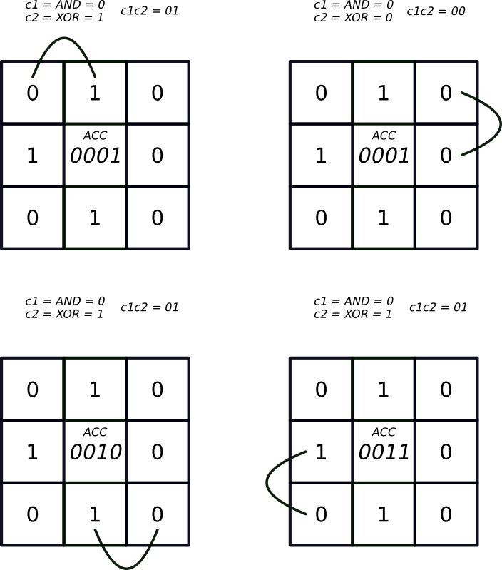
This code is relatively straightforward: for each bit of the result, we perform a XOR operation with either the input aor the carry, and compute the next carry via an AND (except for the last bit, where no carry is needed). All operations are performed homomorphically thanks to the server key.

One element which may surprise readers who aren’t familiar with Rust (or C++, which uses a similar notation) is the use of the ampersand (&). This is used to pass objects by reference rather than by value; a function with an argument starting with an ampersand takes the memory address of the object to find it when needed, rather than creating a new object or moving it. (The details are, of course, a bit more involved than that. For the interested reader, the Rust book provides a good introduction to how objects can be passed to functions in Rust.) Contrary to C++, in Rust the ampersand must be specified both in the function declaration and when called.

Another peculiarity of Rust compared with other popular low-level languages is that a return statement is not always needed. Specifically, if the last line of a function is an expression which does not end with a semicolon, then the value of this expression is returned.

We can now use the above function to write the second part, the accumulator which sums a sequence of encrypted bits modulo 8:

// sum a sequence of ciphertexts, with the value 8 identified with 0
// This function panics if `elements` is empty.
fn sum(server_key: &ServerKey, elements: &Vec<&Ciphertext>, zeros: &(Ciphertext, Ciphertext, Ciphertext)) 
    -> (Ciphertext, Ciphertext, Ciphertext) 
{
    let mut result = add_1(server_key, elements[0], zeros);
    for i in 1..elements.len() {
        result = add_1(server_key, elements[i], &result);
    }
    result
}

Again, this function is fairly straightforward. It takes as arguments a server key, a vector of ciphertexts, and a tuple of three encryptions of 0. It then defines the result by summing the first element with zeros, accumulates the other elements, and returns the result. Notice that this function will crash (or ‘panic’ in the Rust terminology) if elementsis empty. This is not a problem in our case as we know that it will always be of size 8.

Finally, the function is_alive below returns an encryption of ‘true’ if the cell is alive after the update, and ‘false’ otherwise:

// a board structure for Conway's game of Life
//
// Fields: 
//
//  dimensions: the height and width of the board
//  states: vector of ciphertextx encoding the current state of each cell
struct Board {
    dimensions: (usize, usize),
    states: Vec<Ciphertext>
}

impl Board {

    // build a new board
    //
    // Arguments: 
    //
    //  n_cols: the number of columns of the board
    //  states: vector of ciphertexts encoding the initial state of each cell
    //
    // If the length of the states vector is not a multiplt of n_cols, the cells on the incomplete
    // row will not be updated.
    fn new(n_cols: usize, states: Vec<Ciphertext>) -> Board {

        // compute the number of rows 
        let n_rows = states.len() / n_cols;

        Board { dimensions: (n_rows, n_cols), states }
    }

    // update the state of each cell
    //
    // Arguments: 
    //
    //  server_key: the server key needed to perform homomorphic operations
    //  zeros: three encryptions of false (which may be identical)
    fn update(&mut self, server_key: &ServerKey, zeros: &(Ciphertext, Ciphertext, Ciphertext)) {
        
        let mut new_states = Vec::<Ciphertext>::new();

        let nx = self.dimensions.0;
        let ny = self.dimensions.1;
        for i in 0..nx {
            let im = if i == 0 { nx-1 } else { i-1 };
            let ip = if i == nx-1 { 0 } else { i+1 };
            for j in 0..ny {
                let jm = if j == 0 { ny-1 } else { j-1 };
                let jp = if j == ny-1 { 0 } else { j+1 };

                // get the neighbours, with periodic boundary conditions
                let n1 = &self.states[im*ny+jm];
                let n2 = &self.states[im*ny+j];
                let n3 = &self.states[im*ny+jp];
                let n4 = &self.states[i*ny+jm];
                let n5 = &self.states[i*ny+jp];
                let n6 = &self.states[ip*ny+jm];
                let n7 = &self.states[ip*ny+j];
                let n8 = &self.states[ip*ny+jp];

                // see if the cell is alive of dead
                new_states.push(is_alive(server_key, &self.states[i*ny+j], 
                                         &vec![n1,n2,n3,n4,n5,n6,n7,n8], zeros));

            }
        }

        // update the board
        self.states = new_states;
    }
}

Example

Here is a simple example of use, with a 6 by 6 board:

fn main() {

    // define the board dimensions
    let (n_rows, n_cols): (usize, usize) = (6,6);

    // generate the client and server keys
    let (client_key, server_key) = gen_keys();

    // compute three encryptions of 0
    // (we could also work with only one; but this is quite fast in practice)
    let zeros = (client_key.encrypt(false), client_key.encrypt(false), client_key.encrypt(false));

    // initial configuration
    let states = vec![
        true, false, false, false, false, false,
        false, true, true, false, false, false,
        true, true, false, false, false, false,
        false, false, false, false, false, false,
        false, false, false, false, false, false,
        false, false, false, false, false, false,
    ];

    // encrypt the initial configuration
    let states: Vec<Ciphertext> = states.into_iter().map(|x| client_key.encrypt(x)).collect();

    // build the board
    let mut board = Board::new(n_cols, states);
    
    loop {

        // show the board
        for i in 0..n_rows {
            println!("");
            for j in 0..n_rows {
                if client_key.decrypt(&board.states[i*n_cols+j]) {
                    print!("█");
                } else {
                    print!("░");
                }
            }
        }
       
        println!("");
        
        unsafe {
            let runtime_and_energy = time_ene();
            println!("Runtime on the Echip so far: {}s", runtime_and_energy.0);
            println!("Energy cost on the Echip so far: {}J", runtime_and_energy.1);
        }
        
        println!("");
        
        // update
        board.update(&server_key, &zeros);
    }
}

This initialises and calculates the same ‘glider’ configuration that we showed pictorially before, a pattern that moves diagonally while keeping its shape.

To be able to see the system evolve, we also need some way of extracting the information each time the system changes. At each iteration, we return a ciphertext that encodes the updated state of the board. The above code also decrypts each of these ciphertexts and prints the result on the terminal (the output thus looks better with a square font). Here is the result:


Optical Acceleration

The above code works on electronic computers; you can try it out for yourself by copying the above gists into a single Rust file and building it (you’ll also need to have a Rust compiler, the FFTW Fast Fourier Transform library and the Concrete library).

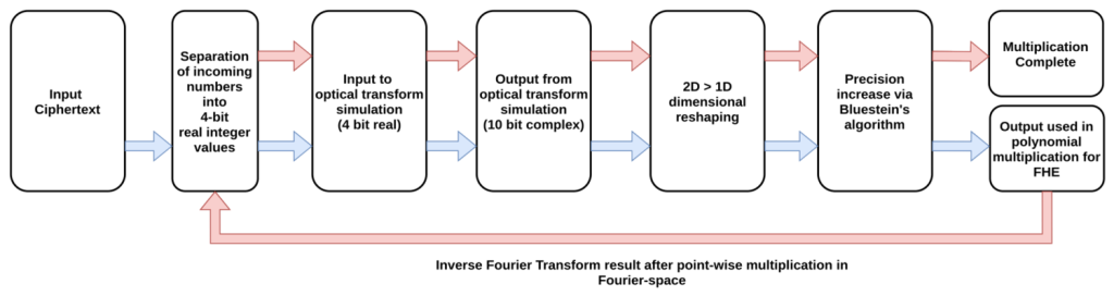
However, as we said above, we aim to demonstrate that key operations in this process can be executed and accelerated by optical Fourier transform hardware. To this end, we also wrote a version of the above code that makes use of a simulated optical Fourier transform and returns performance benchmarks.

The simulated optical Fourier transform

In previous articles, everything we’ve done has used results from physical demonstrator hardware to perform calculations. In this article, we’re using a simulator written in support of our beta program to execute the calculations. This is mainly because executing a serious amount of FHE already requires intensive resources; doing so using the current demonstrator system (which uses thermal modulators that operate in the kHz range) would be slower still, so here we reach for a compromise between speed and accuracy.

This simulator also uses the software interface designed for the physical system, and will be available to partners on our beta program for benchmarking and testing applications.

At the heart of the simulation is a 2-dimensional complex Fourier transform executed to 10 bits (signed 4-bit real and imaginary values) of precision. The raw value also contains an amount of simulated optical noise representative of what we see in real optical Fourier transforms. We then take this value and process it according to the steps we’ve described in previous articles for re-shaping and increasing the precision of an optical transform.

Performance

We executed the Game of Life FHE model as described in the previous section, but with the simulated optical Fourier transform process used in place of the standard FFT function used by Rust. The only difference to the code is made through the use of a custom version of Concrete where the call to execute the Fourier transform is replaced with a call to the custom FT function.

This custom version is somewhat slower than the original, for two reasons. First, since the optical device is fundamentally different than a CPU, the optimal way to perform a Fourier transform on the former is not optimal on the latter. This is because our current optical device effectively works with a radix-49 decomposition for the FFT algorithm (climbing to radix-121 for the final hardware design), while CPUs tend to work better with radix-2 or 4 decompositions. Second, we need to simulate the behaviour of the optical device, which takes longer than just computing a Fourier transform in the usual electronic fashion.

But the speed of our customised version of Concrete is not directly relevant here: our goal is not to develop a faster version of this library (simulating a non-electronic device would certainly not be the right way to proceed), but to estimate how fast it can run using an optical Fourier transform chip operating with the speed and efficiency of the architecture we have developed. Based on these parameters and the results from our simulations, there is good news here: the system could execute the Game of Life demo much faster than a CPU or GPU!

To be more specific, for the 6 by 6 glider example, a modern CPU (Intel i7 @ 3.6GHz) takes about one minute per iteration. Most of this calculation is expended in executing the Fourier transforms needed for efficient ciphertext multiplication. By comparison, an optical device running at 1GHz (the target frequency of our design) would take less than a second to perform the Fourier transforms required for each iteration. We can thus expect to reach a speed-up of a factor of 60, simply by using the optical Fourier transform in place of the electronic one!

In practice, the speed-up for the whole calculation will be smaller because other operations will become the limiting factor. Eliminating the Fourier transform as the primary bottleneck will introduce memory access rates as the limiting factor to FHE, although this is a problem that can be addressed through engineering; overcoming the fundamental limits of the electronic Fourier transform is considerably harder, and our technology is the only hardware that can achieve this improvement.

Taking these caveats into account, we can realistically expect an order-of-magnitude improvement. And this is just the beginning: greater improvements in speed and efficiency will be realised with next-generation optical devices and software improvements that make better use of the optical Fourier transform.


Appendix: A brief intro to FHE (and why it’s currently so slow)

We’ve described why FHE is so slow in some detail in a previous article, but here’s a quick(ish) introduction that describes what FHE is, how it works and what that means for calculations.

  • Most encryption schemes don’t preserve the property of homomorphism. Under most encryption schemes, adding or multiplying pieces of encrypted information will not return the correct output on decryption. This is possible under FHE.

  • If you add or multiply two pieces of encrypted data together within an FHE scheme, then when the result is decrypted it should be the same as if you added or multiplied two unencrypted pieces of data together. (Note, however, that the encryption and/or multiplication in encrypted space may be more complex than the usual ones.)

  • If you can perform additions and multiplications, you can perform the basic operations of Boolean algebra on the data. Ultimately this allows you to perform any sequence of circuit operations that a CPU would, but on encrypted data.

  • This is inherently slower than working on unencrypted data, with the bulk of the computation lying in the multiplication of large polynomials. However, to make matters worse, we have to contend with noise.

  • Practical FHE schemes are built on some variation of the learning-with-errors problem, which means that some noise has to be added to the information as part of making it secure.

  • Adding or multiplying encrypted data increases the amount of noise present in the information. If this noise becomes too large, the data cannot be decrypted. This would impose a limit on the depth of the circuit you can construct.

  • To get around this problem and allow fully homomorphic encryption, you can construct and run the decryption circuit for the scheme using homomorphic operations.

  • This process “decrypts” the data you are working on into a form that is still encrypted, but reduces the noise back down to a manageable level. This process is called “Bootstrapping”, and allows us to evaluate circuits of arbitrary depth.

  • However, now you have to keep executing that decryption circuit repeatedly to manage the noise. This makes FHE even slower; generally speaking, it’s about a million times slower than working on unencrypted data.

So how can we speed this up? Fortunately, where optical computing is concerned, there’s a very easy win.

Optical Fourier transforms for FHE

Most FHE schemes use a variant of the ring-learning with errors problem known as ring-learning with errors (RLWE), where data is expressed as the coefficients of polynomial functions. This makes the ciphertexts a bit more compact and means that all the multiplication steps involved are polynomial multiplications; these can be efficiently accelerated by using the Fourier transform and the convolution theorem.

This is well-established; most FHE libraries and tools already require that a dedicated fast Fourier transform library be installed. TFHE (the basis for Concrete) advises the use of FFTW3, which stands for “The Fastest Fourier Transform in the West (version 3)”. However, while these libraries are highly optimised, they’re still limited by the algorithmic complexity of the electronic FFT.

Despite this limitation, executing Fourier transforms is still more efficient than the naive polynomial multiplication approach (the method typically taught in schools, where the number of operations scales quadratically with the size of the polynomials). While more efficient, this is still remarkable expensive; between 70–90% of the computational work done in executing a sequence of FHE calculations is taken up just by calculating the Fourier transforms!

If you have a very fast, very power efficient optical computing system for executing the Fourier transform, you can vastly accelerate these calculations in a way that no other hardware can. An individual optical Fourier transform is nearly instantaneous and is an O(1) operation, which means that the time taken to perform the task doesn’t increase even as you add more data points to the calculation.

A system that executes a billion 11×11 optical Fourier transforms every second (and can rapidly recombine and reshape the results into an arbitrary transform) can blast through the bulk of the calculations required for FHE faster than any corresponding electronic device. Even systems designed for mass parallel computation (such as GPUs) are at a disadvantage; not only do these systems still need to perform an electronic Fourier transform, but they also need sufficient data to be passed to the system to make effective use of the parallel cores.

That works for the kind of multiplications you might do for deep learning (we can also accelerate that too, by using the same convolution theorem principles that we apply to FHE to eliminate excess operations in certain deep learning network types), but FHE ciphertexts typically aren’t so large that GPUs are tremendously useful, certainly not to the extent that they need to be to make FHE a practical reality. By contrast, an optical Fourier transform system is effectively an extremely fast serial device, delivering maximum performance under a broader range of computational loads.

In summary, the optical Fourier transform approach is a uniquely powerful tool not just for FHE, but for any process where rapid, large scale Fourier transform calculation is either essential (e.g signals analysis and telecoms) or useful (convolutions).

Subscribe

Sign up with your email address to receive news and updates from Optalysys.

Please enable JavaScript in your browser to complete this form.
We respect your privacy.