
We’ve described before how our optical computing system has some inherent advantages over electronic methods when it comes to executing the Fourier transform. Beyond questions of speed or efficiency, because we’re performing calculations using a near-instantaneous 11×11 optical Fourier transform as a basic element (corresponding, more or less, to a radix-121 decomposition), we can cut down on the fundamental algorithmic complexity of this process.
What we’re now covering in this article is the second half of a bigger picture, the question of how we can use a physical Fourier transform of a given size and shape to compute arbitrary digital transforms. We’ve already laid out how we can use this ability to construct larger Fourier transforms in terms of spatial dimension, but thus far we haven’t addressed the question of precision.
Precision in a result matters. Without it, calculations can return answers which are badly wrong. Ensuring the precision of the results returned by our optical system is critical to everything that we see the system being used for.
Combined with our prior work on extending the size and dimension of the transforms we can process, we can now comprehensively demonstrate how the Fourier-optical method of calculation can be used to construct a general-purpose Fourier transform processor of tremendous efficiency.
How efficient? Top-range electronic hardware for mass Fourier transform calculation can perform approximately 3 billion 64-bit operations per Joule of electrical energy transferred to the system. The combined optical-electronic architecture that we are developing can improve on this by a factor of more than 4!
When it comes to an entirely new form of computing, the rules which governed precision in previous technologies can no longer be assumed to hold. In this article, we provide rigorous mathematical demonstrations alongside illustrations that lay out the rules for ensuring that the output of a Fourier-optical computing system is both correct and accurate.
The method we adopt is not just highly efficient from a computational perspective. It also gives us immense flexibility with respect to different applications, as it allows us to provide accurate results at any precision. This allows us to work to the desired precision of any host system where ultra-fast transforms are needed with no changes to the optical architecture.
This is a long article, and it may be that not all of it is of interest to every reader, so we provide links to the different sections below.
In an electronic context, precision refers to the number of bits that are used to describe a number. For example, a 4-bit binary value can represent 16 (2⁴) different levels in base 10 representation.
Performing calculations to a given precision in digital systems is notionally a solved problem. In practice, precision (and more generally how numbers are represented in computers) is still a subject of ongoing development, especially in an age where advances in silicon feature size have slowed.
In recent years, this has led to a move towards low-precision computing in certain applications as a way of getting more effective performance out of a silicon manufacturing node. The advantages are immediate; lower-precision values require far less hardware real estate in terms of logic elements, memory and bus width, thus allowing more the performance of more parallel operations with the same number of components. In a world where the OPS rate is an important metric, that’s a big deal.
This move has been performed alongside research into the suitability of low-precision representations. The findings can be surprising; even 4-bit numerical representations have been found to be suitable for some AI networks.
However, this research has been performed in purely digital systems. Our optical computing system is at heart a kind of analogue computer. Analogue values are continuous; they don’t take discrete levels, but represent numbers to an arbitrary degree of precision. In our case, we use the intensity and phase of light as a way of representing complex numerical values and performing calculations on them. Notionally, these properties of light can take any value, which would pose a problem for digital systems that can only accept a limited range.
In practice, because we are encoding digital values into the light, we should be able to extract discrete values from the output. This is still true, but we face a couple of unique challenges:
1. One of the properties of the Fourier transform is that the output of the transformation of a step function is a spatially continuous function that must be accurately sampled.
2. The fundamental mathematics behind the Fourier transform mean that the values we retrieve are often irrational, and therefore difficult to quantise.
We need a way of overcoming both of these problems. Fortunately, they’re quite closely related, which means that we can develop a solution that addresses both at the same time.
Let’s start from the basics:

The Fourier transform of a step-function (left) is a continuous sinc function in frequency space (right). This is an inherent property of the Fourier transform, not a consequence of analog computing.
If we consider an input grid of spatially discrete sources of light (with perfect fill-factor of the grid), we can see from the above that the output of these points will be continuous even with discrete inputs in terms of amplitude.

A 2-dimensional grid of discrete input amplitudes.

A 3D representation of the above; discrete amplitudes (represented by height and colour) over discrete spatial locations
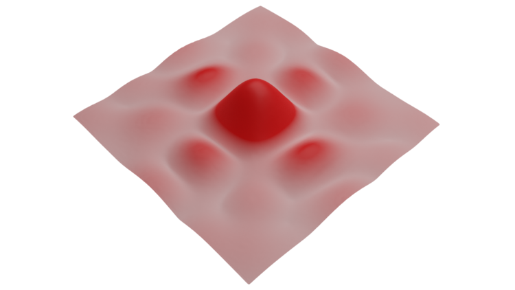
The continuous Fourier transform of the discrete values. Ensuring that this is correctly quantised into a digital signal is not trivial; any errors will grow if the result is used as part of a higher-precision calculation
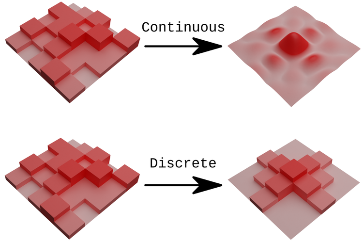
The problem that we’re trying to solve in this article: how to go from a discrete input to a discrete output in an analog optical computing system such that we can reliably build higher precision in a result.
Then, even in the presence of noise or other aberrations that might otherwise flip a bit the wrong way, it should be possible to correctly assign each signal to the corresponding bit-value.
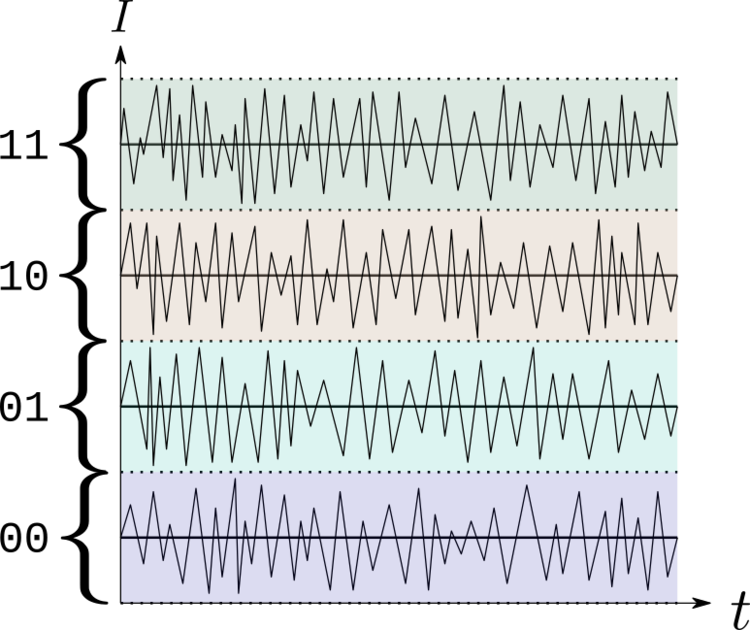
Quantised 2-bit outputs with some optical noise; as long as the noise falls within half the distance between levels, we can successfully assign each signal to the correct digital representation.
The above has important implications if we want to be able to increase the precision of a calculation. There is a technique that we can borrow from digital electronics called bit-shifting that allows us to do this, but attempting to use bit-shifting without addressing the above can lead to errors which grow exponentially at each iteration.
We need a solution to this; one which overcomes this problem in a way that yields results which are both correct (returns the output we would expect for a transform executed to the same precision in a digital system) and deterministic (sending the same input several times should yield the same outcome) when the output of an optical Fourier transform is converted into a digital representation. One which is also fast, and doesn’t hinder the advantage that optics can provide.
Is there such a solution? There is. In this article, we lay out how we can use the properties of convolution to ensure that these conditions are met.
First, let’s start with a description of how we can reconstruct a higher precision digital result from operations performed in a lower-precision system. Doing so involves manipulating the properties of binary numbers. Consider a binary value such as
110011100110 = 3302
The individual values running from left to right represent decreasing powers of 2; we can re-assemble the base-10 value represented by this binary value by adding these powers of two together.
100000000000 = 2¹² = 2048
010000000000 = 2¹¹ = 1024
000010000000 = 2⁸ = 128
000001000000 = 2⁷ = 64
000000100000 = 2⁶ = 32
000000000100 = 2³ = 4
000000000010 = 2¹ = 2
2048 + 1024 + 128 + 64 + 32 + 4 + 2 = 3302
We can further manipulate this property; for example,
1100 + 0001 = 1101
is normally equal to (8+1 = 13), but if we then shift that value to the left by 4 places (here, we do this simply by adding zeroes on the right), this changes the value of the result
11010000 = 208
This is the same as directly adding
11000000 + 00010000 = 208
Alternatively, if we then perform another operation on a pair of 4-bit values, e.g
0101 + 0011 = 1000 (5+3 = 8)
we can append this result to the end of the first value as we shift it left, resulting in
11011000 = 216
which is equivalent to writing 208 + 8 = 216.
The above process is also equivalent to directly adding 11000101 and 00010011 together! If we can only work on a limited number of bits during an operation, this gives us a way of building up the precision in a result. However, this is only possible if the operation we are performing is linearly separable. Here’s what that means for Fourier transforms.
Consider a set of values arranged over a 2-dimensional grid.
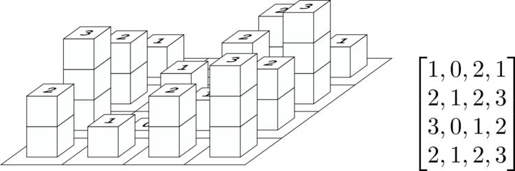
We can take the Fourier transform of this grid directly, or we can separate this grid like so…
…and then perform the Fourier transform on each sub-grid, before summing the results to retrieve the Fourier transform of the original grid. The values over which we perform the Fourier transform can thus be linearly separated; you can check this property using the following gist:
# Linear separability in Fourier transforms

# A simple example of linear separability in the Fourier transform.

import numpy as np

grid_original = [[1,0,2,1],
                [2,1,2,3],
                [3,0,1,2],
                [2,1,2,3]]

subgrid_1 = [[1,0,1,1],
            [1,1,1,1],
            [1,0,1,1],
            [1,1,1,1]]

subgrid_2 = [[0,0,1,0],
            [1,0,1,1],
            [1,0,0,1],
            [1,0,1,1]]

subgrid_3 = [[0,0,0,0],
            [0,0,0,1],
            [1,0,0,0],
            [0,0,0,1]]

ft_grid_original = np.fft.fftshift(np.fft.fft2(grid_original))

ft_subgrid1 = np.fft.fftshift(np.fft.fft2(subgrid_1))

ft_subgrid2 = np.fft.fftshift(np.fft.fft2(subgrid_2))

ft_subgrid3 = np.fft.fftshift(np.fft.fft2(subgrid_3))

ft_linear_recombination = ft_subgrid1 + ft_subgrid2 + ft_subgrid3

print("Fourier transform of original grid: \n" + str(ft_grid_original))

print("Reconstructed transform from linear recombination: \n" + str(ft_linear_recombination))
The exact result for the above is also an integer-valued complex number.¹ If the system is deterministic and the outputs are also expected to be integers, then we can use linear separability and bit-shifting indefinitely for greater precision in the Fourier transform.
But what about the case where we’re working with floating-point numbers, the standard digital method for representing decimal values (e.g 1.156832)? These come up quite frequently in mathematics and we have to be able to account for them in our system. We also need to account for them if the size of the Fourier transform in one direction is larger than 4, as even an integer-valued input will then yield (except in specific cases such as a uniform input) a complex-valued output with irrational real and imaginary parts.
Fortunately, this is a simple process; most programming languages do this automatically (e.g. Python, Julia, and C/C++) or explicitly (e.g. Rust), allowing mixed use of floats and integers with conversion performed as needed. Here’s how this is done in electronic systems:
The integer is converted into a representation in terms of the sign(positive or negative) and a binary representation which is always positive.
This positive binary number is then converted to a fixed-pointrepresentation by shifting the decimal point (hence the “floating-point” name) to the right of the most significant bit in the binary value.
The number of times the decimal needs to be shifted is called the exponent. The binary value to the right of the decimal is now known as the mantissa.
The exponent is expressed in an offset-binary representation.
The floating-point value is represented as a combination of the sign bit, the exponent, and the mantissa
This operation can be performed very quickly in digital systems. Floating-point values can be converted to integers, processed optically, bit-shifted and converted back into floats much faster than performing the Fourier transform directly on a grid of floats. Despite operating on two different types of number, the outcome of the above methods is identical.
However, all the above is dependent on ensuring those vital conditions of determinism and correctness in the result, so let’s now take a look at how we ensure this.
In this section, we show how we can solve the discrete-to-discrete mapping problem for an analogue-optical Fourier transform. This algorithm can actually be used to compute a more general transformation called the chirp z-transform.
Chirp-z transforms are a generalisation of the discrete Fourier transform. Before we explain what this means, we first consider the term highlighted in the discrete Fourier transform equation below:

This term represents a “complex root of unity”, complex-number solutions to the equation

for some positive integer n. The complex roots of unity all lie on the same circle in the complex plane, called the unit circle, with centre 0 and radius 1.

Complex roots for n=6 lying on the unit circle
The symmetries in the complex roots of unity are the key to understanding the utility of most Fast Fourier transform algorithms, as it is this symmetry that allows the FFT to cut down on what would otherwise be duplicate calculations in the discrete Fourier transform. However, this also presents a problem for precision limited systems; the complex roots of unity (when expressed in the usual a + bi form of representing complex numbers) generally² have irrational coefficients.
To relate this back to an optical Fourier transform calculation, what we are detecting at the photodiode array is also a complex number in the form a + bi, where the values of a and b are determined by the quantisation of the photocurrent. However, attempting to quantise an irrational value with a limited number of bits will introduce a source of truncation error into the result. If we then bit-shift these results, the magnitude of this error will also grow to the same scale as the maximum shift.
A “pure” complex number. The real and imaginary parts can have irrational values.
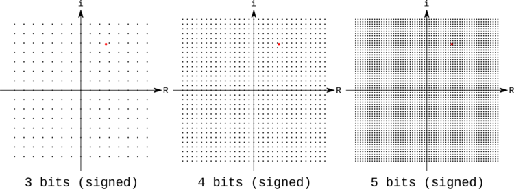
The same complex number relative to the discrete grid of points that can be represented with increasingly large binary value representations of complex numbers. The distance between the “true” complex value and the nearest grid point represents a source of inaccuracy known as a truncation error; this error decreases as the precision of the result in bits increases.
We can see in the above that increasing the precision of the result will reduce the truncation error, but what do we do if we need to increase this precision through bit-shifting? Bluestein’s algorithm gives us a way of overcoming the truncation error by re-phrasing the Fourier transform in terms of a discrete convolution. Since this can be used to compute any chirp-z transform using an optical system, we first briefly describe this transformation, which has its own set of applications.
Formally, a chirp z-transform is a function that takes a complex-valued vector as input and returns another complex vector, obtained by summing its coefficients with weights given by powers of some fixed complex number. More precisely, the chirp z-transform of input size N and output size M with parameter z, where N and M are positive integers and z is a complex number, is the function defined by:

Notice that, if M = N and z = exp(-2 i π / N), cz(x) is a discrete Fourier transform of x. In this sense, chirp z-transforms are direct generalisations of discrete Fourier transforms.
As with the DFT and the complex roots of unity, they may be understood geometrically as follows: a chirp z-transform corresponds to summing the components of a vector multiplied by weights which are distributed on a logarithmic spiral in the complex plane, with a fixed angle difference between two consecutive points and starting from 1.
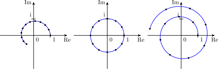
Illustration of the effect of changing the parameter z on the chirp z-transform for N = 12. Black dots show the positions in the complex plane of the powers of z by which the coefficients of the input vectors are multiplied, and the blue line materialises (part of) the logarithmic spiral where they are located. In the middle panel, z has modulus 1 and its phase is an integer fraction of 2π. Its powers are then regularly spaced on the circle with centre 0 and radius 1, and the chirp z-transform is equivalent to a discrete Fourier transform. In the left and right panels, the modulus of z is, respectively, smaller than and larger than 1, and its phase is not an integer fraction of 2π. The corresponding transformation is thus different from the discrete Fourier transform.
In the next few sections, we show how the chirp z-transform (and thus the discrete Fourier transform, as a particular case) can be reformulated as a convolution. This is a bit more technical, so at the end of this article we also provide a visual interpretation that ties everything together.
The reason we may want to re-phrase the chirp z-transform as the outcome of a convolution is that we can then ensure that the results fit into known quantisation bands, eliminating the potential for error. Of course, any optical noise present in the result will also be carried forwards with the convolution, but as described previously this can be accounted for in the quantisation scheme.
This rephrasing can be efficiently performed using an algorithm attributed to Leo Bluestein, often referred to as Bluestein’s algorithm. When used in conjunction with the ability of the optical system to perform an instantaneous Fourier transform, this approach allows us to compute a chirp z-transform or discrete Fourier transform with an arbitrary level of precision.
In the following, for simplicity we will assume that the input size N and output size M are equal. It can easily generalise to different values by either padding the input with zeros if M > N or truncating the output if M < N.
The main idea of Bluestein’s algorithm is to rephrase the chirp z-transform as a convolution with periodic boundary conditions, which can be performed efficiently using Fourier transforms. It relies on a very simple observation: for any two integers m and n,

Using this identity, it is easy to show that, for all complex vectors x with Nelements and all integers m between 1 and N,

So far, this formula looks more complicated and less useful than the definition of the chirp z-transform. But it can be greatly simplified.
To achieve this, we first need to define a few things. For each positive integer L, we define the two operations ⚬ (element-wise multiplication) and ⊛ (periodic convolution) on complex vectors with L components as follows: for any two such vectors and each integer l between 1 and L,

and

We also choose a positive integer K no smaller than 2N-1 and define the following two vectors:
a vector with N elements containing the relevant powers of z:

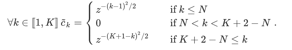
a vector with K elements which contains the relevant negative powers of z as its first N components, the inverse powers of z in reversed order as its last N-1 components, and is padded with zeros:
Finally, we define the padding function P (input: N-components vector; output: K-components vector) and the truncation function T (input: K-components vector; output: N-components vector) by:

and

Then, for each complex vector x of size N, we have

This means that the chirp z-transform of an input x can be computed in 5 steps:
Compute the element-wise product of x with c.
Pad the result with zeros to size K.
Compute the periodic convolution with a pre-computed vector.
Truncate the result to size N.
Compute the element-wise product of the result with c.
We mentioned previously that we can use Bluestein’s algorithm as an efficient tool for executing the chirp-z transform; let us now take a moment to estimate the complexity of each of the steps covered above.
Steps 1 and 5 involve N-1 complex multiplications each (technically N, but the first component of the vector c is 1, so there is no need to perform the multiplication explicitly). This can be done with either 4 (N-1) real multiplications and 2 (N-1) real additions, or 3 (N-1)real multiplications and 3(N-1) real additions.
Step 2 requires us to append K-N zeros to a vector. In practice, one may directly store the result of step 1 in a larger array pre-filled with zeros. Step 4 simply involves reading N elements from an array. So, steps 1, 2, 4, and 5 all have a linear complexity in K.
Step 3 is the real bottleneck. Indeed, the convolution of two vectors with length K, if performed using the above definition, requires (K-1)² complex multiplications and K (K-1) complex additions. Except for the smallest values of K (and thus of N), this is much more demanding than all the other steps combined.
Fortunately, it is possible to significantly reduce this complexity using Fourier transforms. Indeed, denoting by F the discrete Fourier transform of size K, we have for any vectors x and y of size K:

Using a fast Fourier transform algorithm, the asymptotic complexity of this operation becomes O(K log K). However, this can itself be efficiently accelerated using Fourier-optical hardware, as detailed in these articles. Notice also that, in Bluestein’s algorithm, one of the two vectors in the convolution is independent of the input x. Its Fourier transform can thus be pre-computed, eliminating the need to perform an additional operation using the optical system.
At this point, it may seem like we are going round in circles: we mentioned that discrete Fourier transforms are a special case of chirp z-transforms, but we now need Fourier transforms to compute the latter efficiently. And, indeed, if all you are interested in is the Fourier transform function F, Bluestein’s algorithm will be of little use to you. There are, however, at least two special cases where it is very useful.
The first one is to compute Fourier transforms of arbitrary sizes. The reason why most fast Fourier transform algorithms such as the Cooley-Tukey algorithm are efficient is that they split the original Fourier transform into many smaller ones and then recombine the results using the symmetries in the complex roots of unity. For instance, if N=2ⁿ for some integer n, one can evaluate a Fourier transform of size N by performing n2ⁿ⁻¹ Fourier transforms of size 2 and as many complex multiplications. The resulting asymptotic complexity is O(N log N), which is much better than the complexity O(N²) of using the raw definition of the Fourier transform. However, this is only efficient if N is the product of many small factors. If N has large prime factors, such algorithms become much less efficient — typically, their complexity (without other optimizations) is at least Ω(p²) where p is the largest prime factor of N.
Bluestein’s algorithm solves this problem by allowing us to evaluate a Fourier transform of size N using Fourier transforms of a different size K, with the only constraint that K be no smaller than 2N-1. For instance, for N = 7919 (which is a prime number), it can be evaluated using Fourier transforms of size K = 16384 = 2¹⁴. While K is larger than N, Fourier transforms of size K are typically must faster to evaluate in practice because they can be decomposed into Fourier transforms of size 2.
The same argument also holds for hardware designed to efficiently compute Fourier transforms with a size different from 2, such as the Optalysys technology: starting from a Fourier transform of size S (and assuming S > 1, of course), a Fourier transform of an arbitrary size N can be computed by using the Cooley-Tukey algorithm to perform Fourier transforms with length equal to the smallest power larger than or equal to 2N-1, then using Bluestein’s algorithm to reduce this size to N.
The second important use case is when the Fourier transform can not be directly computed with the desired accuracy. Indeed, Bluestein’s algorithm allows us to compute Fourier transforms with an arbitrary level of accuracy by using a base convolution function with a finite accuracy. Let us sketch how this works.
We focus on the convolution step of Bluestein’s algorithm, as this is the main bottleneck in the process and the one which uses Fourier transforms. The convolution has three important properties:
It is a bilinear function, i.e., it is linear in each of its inputs.
It maps integer vectors to integer vectors: if x and y are two complex vectors with the same number of elements and if the real and imaginary parts of each coefficient of x or y is an integer, then each coefficient of x ⊛ y also has integer real and imaginary parts.
It is bounded: if x and y are two complex vectors with the same number K of elements, and if the absolute values of the real and imaginary parts of each element of x and y are smaller than some number M, then the absolute values of the real and imaginary parts of each element of x ⊛ yis smaller than K M².
We’re especially interested in the second point, which allows us to map discrete integer inputs to discrete integer outputs despite the irrational numbers which appear in the Fourier transform.
The second and third properties imply the following: if each coefficient of xand y can be represented with b bits, where b is a positive integer, then each coefficient of x ⊛ y can be represented exactly with 2b+2 + ⌈log N⌉ bits (or 2 + ⌈log N⌉ if b = 1), where the logarithm is in base 2. The last term can be reduced if x or y has some vanishing coefficients.
To return briefly to our earlier description of the chirp-z transform, note that this property does not apply to the generic Fourier transform: since the DFT involves multiplications by complex numbers with irrational real and imaginary parts (except in the particular cases of size 1, 2, or 4), the second property above is not satisfied, and the output will generally not be representable exactly with a finite number of bits even for integer inputs.
Let us now see how this can be used to increase the accuracy of the convolution performed by a finite-precision compute device.
Let x and y be two vectors. Assume we wish to compute their convolution with b₁ bits of accuracy for both the input and output, using convolution hardware (for instance, an optical Fourier engine with additional logic to perform the component-wise multiplication) with b₂ bits of accuracy, where b₂ < b-1. For simplicity, we assume that b₂ > 2 + ⌈log N⌉.³
One possible strategy is the following (note that it can be adapted and optimized for specific workflows, e.g. if the required accuracy on the input and output are different, or to use powers of an integer different from 2):
Find two scale factors sₓ and sᵧ such that the integer parts of each coefficient of sₓ x and of sᵧ y is accurate to b₁ bits. Define the vectors x̄and ȳ by discarding the fractional parts of the real and imaginary parts of sₓ x and sᵧ y, respectively.
Decompose x̄ and ȳ into vectors with at most b bits per real or imaginary part of each coefficient, where b is a positive integer such that 2 b + ⌈log N⌉ < b₂ if such an integer exists, or b = 1 otherwise, so that

and

3. The convolution of x and y (the output of which is, as a reminder, the discrete Fourier transform or chirp z-transform that we seek) can then be computed using the formula:
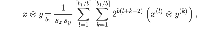
where each of the convolutions now only involve real numbers with at most b₂ bits (and can thus be computed using the convolution hardware), and the b₁ under the equal sign means ‘equal within b₁ bits of accuracy’.
If x is a vector of outputs from the detection of an optical Fourier transform, the above convolution process will (via the properties of the chirp-z transform) thus produce an output which is exact with respect to the precision of the detection scheme!
We’ll now tie together everything we’ve outlined above using a visual perspective.
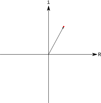
Let us say that we have already computed a Fourier transform to a high degree of numerical precision. For illustrative purposes, we select one of the values of this output and display it in complex space as a red dot.

Let us now assume that we want to use a precision-limited optical device and bit-shifting to perform the same transform to the same degree of precision.
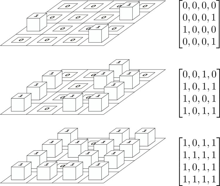
Using the property of linear separability in the Fourier transform, we can feed the input value into the system as separate “frames” of bit-words which are then encoded into light and emitted into the free-space processing stage of our system, with the Fourier transform of these values being detected by the receiving side of the system.
In this example, for the purposes of visualisation, we assume a device capable of 2-bit signed complex output. In practice, the system we are developing has a higher output precision.
In the following, we pick the same output value from the high-precision Fourier transform to focus on. The complex binary outputs closest to this value are represented as a green dot. The purpose of Bluestein’s algorithm can be summarised as ensuring that the quantised outputs of the optical Fourier transform correctly “snap” to these values every time.
For each frame that we pass through the system, the use of bit-shifting means that we are effectively “zooming in” to the region that contains the higher-precision result on each frame.
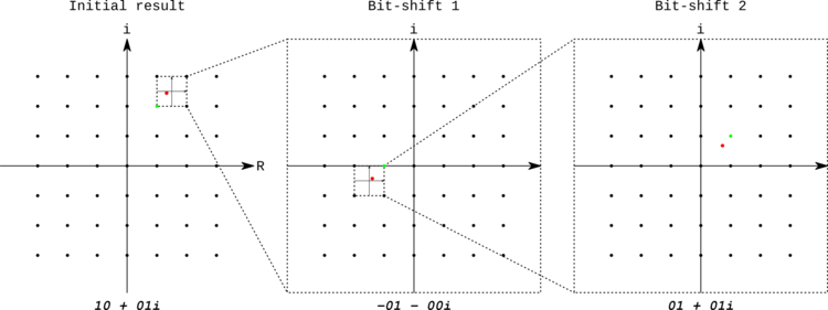
It may not look like the precision of the result is increasing in the above, but if we instead stack the output of each frame, scaled and positioned relative to the last…

… we can see that outputs of each frame are indeed steadily converging on the correct answer. Because the Fourier transform is linearly separable, we can then bit-shift the results to retrieve the higher-precision binary value:

Bit-shifting and summation of the results. In practice, the negative values wouldn’t be subtracted, but would instead be represented in two’s complement form and then added.
Using this algorithm and the methods outlined above, discrete Fourier transforms with arbitrary accuracy can be efficiently obtained from finite-precision analog hardware. Furthermore, this technique can be efficiently combined with the method of calculating larger Fourier transforms of different size and dimensions to the optical output, allowing for the construction of a general-purpose Fourier transform engine that can execute results to arbitrary size and precision.
The above methods make it possible to reliably increase accuracy when digitising an optical Fourier transform. But what additional overheads does this pose for the efficiency and speed of the optical method?
This is a crucial question. In this section, we break down the process outlined above to give an overview of what this means for performance relative to other approaches to calculating the Fourier transform.
Our system as designed passes a full frame of data through the optics at a rate of 1 GHz; 1 11×11 frame every nanosecond. The precision of the input is a 4-bit real value; the native precision of the result is a 10-bit complex number with signed 4-bit real and complex components.
The algorithmic complexity of reconstructing a larger Fourier transform using a base 2-dimensional optical transform can be shown to be:

where nx, ny are the x and y dimensions of the base 2D grid. Precision can be built in a large-transform result obtained using this technique by using the same methods described in this article for a native 11×11 grid.
With respect to the complexity of boosting precision, we’ve already given a breakdown of the algorithmic complexity of Bluestein’s algorithm in the section on complexity considerations, in which we demonstrate that the asymptotic complexity of Bluestein’s algorithm is notionally O(K log (K)) where K is the size of the x and y vectors in the convolution. This is a consequence of the complexity of the electronic Fourier transform; however, we have access to an O(1) optical transform. As the other operations in Bluestein’s algorithm are linear in time, we can therefore use the optical system to perform the transforms involved in the convolution, reducing the overall complexity to O(K).
Normally, this process would involve 2 forward Fourier transform operations and an inverse transform, all performed in optics. However, as one of the forward transforms is static and can be pre-computed, this further eliminates an additional optical pass.
So how many frames (or, more usefully for transforms of arbitrary dimension, distinct layers of additional transformation) do we require?
It’s helpful to use a transform of a given size to set some benchmarks; here we choose to estimate the evaluation of a 1331×1331 transform to 60-bit complex precision using a device with a native 11×11 grid working with 10-bit complex numbers. There are three main steps we need to consider.
First, the 1331×1331 input grid needs to be decomposed into 11×11 ones. This yields 121×121 = 14641 sub-grids.
Second, the results of the smaller Fourier transforms need to be combined to reconstruct the 1331×1331 Fourier transform. As we sketched in this article, this can be done using a two-dimensional equivalent to the Cooley-Tukey algorithm, which requires 3 optical frames for each sub-array.
Finally, each of the 60-bit inputs need to be split into 10-bits slices. This step multiplies the number of frames needed by 6²+6 = 42.
The total number of frames needed to process the result to the required precision is thus 14641×3×42 = 1,844,766. This may look like a lot, but the equivalent on an electronic system requires about 183,857,824 64-bit operations!
So what does this mean in the context of the hardware that we’re developing? We’ll have a dedicated article out soon on the specs of our system, but we can openly state some of them here.
The optical computing architecture that Optalysys are developing will process 1,000,000,000 optical frames per second, corresponding to a processing speed of 99.7 giga-operations per second. The power draw of the core architecture is just 2W; since we intend to use 4 Etiles to process fully-complex inputs, this yields a normalised processing efficiency of 12.5GopJ (giga operations per Joule). By comparison, the best current Fourier transform hardware for mass FT calculation can perform at about 3GopJ for the same operation.
Not only is this a massive improvement over electronic systems (even at higher precision!), but the combination of speed and the calculation methods we’ve adopted means that the precision of a result can be controlled by software without losing either the speed advantage or wasting architectural real-estate. This means that an optical approach isn’t just suitable for making a general-purpose Fourier transform processor, it also allows us to make the best FT processing core possible.
We’ve been developing our next-generation optical system for some time now. In our next articles, we’ll be releasing details not only on the operating parameters of the core architecture, but our intentions for making them a reality on the mass production scale.
Until then, you can read other articles on www.optalysys.com for more information on what we’re up to.
¹ This property is specific to Fourier transforms of size 1, 2, or (as in the present case) 4 in each direction. For other sizes, the Fourier transform of an array of integer will generally involve irrational numbers.
² Except for n = 1 (the only root is 1 itself), n = 2 (the two roots are 1 and -1) and n = 4 (the four roots are 1, -1, i, and -i).
³ If that is not the case but b₂ > 1, one can first write x as a sum of several vectors with at most k coefficients each, where k is a positive integer such that b₂ > 1 + ⌈log N⌉, go through the algorithm with x replaced by each of these vectors, replacing N by k, and sum the results.
News
© 2024 All rights reserved Optalysys Ltd
Subscribe
Sign up with your email address to receive news and updates from Optalysys.