
In our previous article on cryptography, we took a look at the concepts behind one of the most popular public-key cryptography schemes, and explained why we need an alternative because of the threat of quantum computing.
The security of one of the most popular public-key encryption schemes, RSA, is based on the difficulty of factoring large primes, a task which is anticipated to be much easier for quantum computers. One of the most promising routes for building quantum-secure cryptosystems is lattice-based cryptography, where the security of the scheme is based on the properties of mathematical objects called lattices.
When we say that a cryptosystem is “lattice-based”, we mean that breaking the security of the scheme can be shown to be fundamentally equivalent to solving certain difficult computational problems on lattices, not that lattices are themselves inherently cryptographically secure. There are many mathematical problems involving lattices which are perfectly solvable.
This might seem obvious, but it’s an important distinction to make. Lattice-based schemes are not secure just because they’re lattice based, and require the same oversight as any other cryptographic scheme. The United Kingdom’s Government Communications Headquarters (GCHQ) developed their own lattice-based cryptographic scheme that they called Soliloquy, only to later abandon it when they realised that there was an effective quantum computing attack against it.
Fortunately, while Soliloquy is an example of a lattice-based scheme that was vulnerable to a quantum attack, it also relied upon a very different “hard” problem to the ones that we’re going to look at today.
In this article, we take a look at the lattice problems which can be used to make cryptographic constructions that aren’t just secure against attacks from quantum computers, but can form the basis of many different types of cryptographic system. Some of these systems can themselves be used to construct ways of performing fully homomorphic encryption, a phenomenally useful concept that can revolutionise the way in which we handle and process sensitive data.
We’ll start by explaining what a lattice is, and then build on that to explain why certain problems involving these structures have the properties that we’re looking for in a mathematical problem on which to base public-key cryptography.
Lattices are mathematical structures that repeat infinitely in space. Here’s a basic 2-dimensional example:

A simple triangular lattice in 2 dimensions. The black dots are the “points” of the lattice; the white space enclosed by the grey lines surrounding each point indicates the area which is closer to that point than any other.
Lattices can have more than two dimensions. Here’s a three-dimensional one:

A 3-dimensional cubic lattice
We can even define a lattice with a higher numbers of dimensions. While we can’t visualise them as easily, they work just the same mathematically.
Because lattices repeat themselves, we can use only a few very basic rules to define where every single point should be, even though they’re infinite in size. For a lattice of n dimensions, we can make this definition using only n “vectors”, collections of numbers that define both a direction and a magnitude. Let’s try this out by making a basic square lattice.
There’s no point in the lattice which is more “important” than any other, so we can pick any position to start with:

We’re working in 2 dimensions, so we only need 2 vectors to define the rest of the lattice. We’re making a square lattice, so the vectors are at right-angles to one another. Starting with our initial lattice point, we can draw vectors out to define the position of two new points, like so:

Then we can use one of these new points and the same vectors to draw out two more new points…

…and we can keep going…
… forever, in principle. Any new point in the lattice can be constructed as a straightforward integer multiplication of these simple vectors, so more generally we can say that a lattice is a set of integer combinations of linearly independent vectors.
This is a very simple concept, but there’s a fiendishly difficult problem hiding in plain sight. It’s called the shortest vector problem.
When we made our lattice, we picked two very simple vectors as the basisfor constructing our lattice. If you’re familiar with Pythagoras’s theorem, you can quickly see that these two were the shortest possible vectors from which to construct the square lattice. However, any lattice (apart from a 1-dimensional one) has an infinite number of possible bases. Take the triangular lattice we looked at earlier:
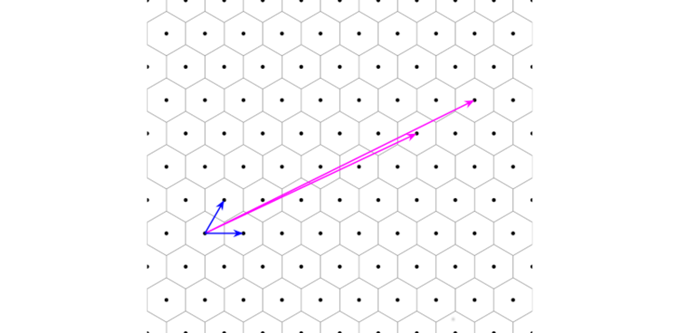
The shortest vectors in the triangular lattice (blue), and two longer vectors (purple). We can use either pair of vectors as the “basis” for constructing the lattice using the same method we described above. The purple vectors are a “bad” basis for building the lattice, while the blue ones (as the shortest vectors) are the most easy to work with.
If we multiply the longer basis vectors by whole numbers, they’ll also land on new points in the lattice. We can therefore use any pair of vectors to make a lattice as long as each vector terminates at a new lattice point.¹ Likewise for the 3-dimensional square lattice:

In principle, we can reconstruct the whole lattice from any basis we are given and find the shortest vectors. In practice, depending on the lattice and the basis vectors we choose, this problem can be very easy or it can be almost totally impossible.
If all the vectors in the basis are very long, finding the shortest vectors requires that we keep taking combinations of the very long vectors to try and reconstruct the lattice. That’s still fairly simple for a 2-dimensional lattice, but if we increase the dimension of the lattice, it becomes difficult.
The reason why this happens is because the number of possible combinations that we have to try increases exponentially with the number of dimensions. If we say that a is the typical length of the vector relative to the spacing of the lattice points and d is the dimension of the lattice, then the number of possible combinations we need to try is on the order of (2a)ᵈ.
For the long bases shown in the 2-dimensional examples above, a is “about 4” and d =2, which from (2a)ᵈ means that we have to try about 64 combinations before we can find the shortest vectors.
If we increase a to 100 and use a 50-dimensional lattice, (2a)ᵈ >10¹⁰⁰ different combinations. For reference, that’s more than the estimated number of atoms in the observable universe.
Of course, we have to be careful with what we’re saying here; there are clever techniques (such as the Lenstra-Lenstra-Lovasz algorithm) that can be used to find short vectors on lattices without trying all the possible combinations. However, it’s still true that the complexity and size of the problem increases explosively with the number of dimensions, such that even the best known algorithms running on the fastest supercomputers cannot find the shortest vectors in high-dimensional lattices in an acceptable timeframe.
Just as large prime factorisation is very easy to undo if you know whichlarge primes were multiplied together and (currently) nearly impossible otherwise, with only 50 vectors we can construct a problem with the same property; it’s easy to solve certain problems on the lattice if you know the shortest vectors and unbelievably difficult if you don’t.
And best of all, there’s no known quantum algorithm for solving this kind of lattice problem.
This is the thing that we were hoping for in the last article [LINK]; something that we can use as a cryptographic trap-door function that will allow us to encrypt something in such a way that we can decrypt it only if we know some other secret piece of information, and it’s also secure against quantum attacks!
This is great; there’s something here that we can use to make (amongst other things) a new post-quantum public-key cryptosystem, but now we need some practical way of using it. Fortunately, while the shortest vector problem is a great introduction to lattice security, it isn’t the only “hard” problem on which to base a scheme.
The two most important computational problems in lattice-based cryptography are the shortest vector problem and the closest vector problem. We covered the basic version of the shortest vector problem above, but we’ll give a few examples of some of the more important variations on the problem.
Search-Approximate
In the search version of the approximate shortest-vector problem, we’re given a lattice and asked to find a vector whose length is within a factor g of the smallest possible value (i.e, whose length is at most g multiplied by the length of the shortest vector)

An example of the search-Shortest Vector Problem. The grey area indicates all the possible vectors which are nearly the same length (to within a given factor) as the shortest vector, which is indicated in blue. The vector in green indicates one of these possible solutions, while the purple vectors indicate a “bad” basis that we are given.
If this factor is 1, the problem returns to being the original shortest vector problem.
Decision-Approximate
In the decision version of the approximate shortest-vector problem, we’re given a number d and asked to determine if the length of the shortest vector is smaller than d, larger than d, or “undetermined”.

The decision-approximate shortest vector problem. d is a real number, shown here by a circle that represents all the possible vectors of length d. The blue vector is the shortest vector.
Closest Vector Problem
The closest-vector problem is the other significant category of computational problems on lattices. In this problem, we’re given a pair of “bad” (long) basis vectors, and then asked to find the lattice vector closest to another vector which isn’t part of the lattice.

Two “bad” basis vectors (purple) and a vector that isn’t part of the lattice (green). The closest lattice point to this vector is also highlighted in green.
This looks easy, because it’s easy to see where the closest lattice point is when they’re all drawn out. Indeed, it is easy if our lattice has a basis set which is orthogonal (at right-angles to one another, as in the case of our square lattice). However, many lattices don’t have an orthogonal basis, and if we take away the points…

…it gets tougher to see the correct solution, and a lot tougher if we increase the dimensions of the lattice.
The closest vector problem also has an approximate version, which can be used to build cryptosystems. It isn’t actually provably secure for all values of the approximation parameter, but it is a very close relative of a related (and demonstrably secure) problem called…
The Bounded Distance Decoding Problem
In the bounded-distance decoding problem (BDD), we’re now given a vector which isn’t in the lattice but does lie within a set distance from a point in the lattice, and we’re asked to find the closest lattice vector.

The bounded distance decoding problem. As in the closest-vector problem, the aim is to find the lattice vector that lies closest to the green vector, where the green vector is known to lie within a given distance (in this case, half the length of the shortest vector in the lattice) from a lattice point.
This is very similar to the closest-vector problem, but as long as we pick an appropriate distance we are now guaranteed that there is a unique solution. When considering the cryptographic side of things, it’s helpful to put this problem in the context of communications theory.
In communications theory, BDD can be used to retrieve information sent over a channel which contains white (random) noise with a Gaussian distribution. The information to be sent is stored in the form of a lattice vector, so the person receiving the message needs to be able to recover this original lattice vector from the noisy version that they receive.

In communications theory, we can pick a lattice vector that represents part of a message, and send it over a “noisy” channel which alters the precise value of the vector. In the above, we can represent this noise as a Gaussian distribution around one of the lattice points; the green region indicates all the places where the vector might be moved to by the noise.
Because we’re now guaranteed that there’s a solution, we can use BDD to recover the correct value as long as we pick a lattice with sensible parameters for a given amount of noise. From the above illustrations, it should be fairly clear that decoding to a “unique” point in the lattice is only possible when the radius of the noisy region is less than or equal to half the shortest vector. We can see this explicitly below, where we show bounding regions which have this maximum radius; if the regions were larger they would overlap, making it impossible to distinguish some vectors as belonging to a specific lattice point.

This might seem like a bit of a diversion, but in fact this combination of Gaussian noise and bounded-distance decoding is fundamental to a very important cryptographic construction known as the Learning with Errors (LWE) problem.
In our next article, we’ll be looking at an application of the learning with errors problem and another important extension of it, ring-learning with errors. This application, known as fully-homomorphic encryption or FHE, is a novel form of encryption that allows us to work on data even when it is encrypted. This means that even highly sensitive data can be sent to a cloud server for processing without ever risking that the data could be compromised.
We’ll be talking about how ring-learning with errors techniques can be performed using a Fourier-optical processing system, and then show how we applied our prototype system to performing encryption and decryption operations in an FHE scheme.
¹ There is an additional condition for the set of vectors to form a basis which is able to generate the whole lattice: the matrix relating it to the original basis must have a determinant equal to +1 or -1.
News
© 2024 All rights reserved Optalysys Ltd
Subscribe
Sign up with your email address to receive news and updates from Optalysys.