
In our previous article on self-driving vehicles, we explored some of the nuances of the two most common algorithmic approaches. These are:
An end-to-end solution – in which a single deep neural network learns to map sensory inputs directly to the appropriate driving response.
A mediated perception approach – in which the driving system is created by combining independent modules that each detect semantic features (e.g. stop signs).
There are strengths and weaknesses to both of these solutions, and both approaches are being attempted by organisations with interests in the field. The tension between the two ideas reflects analogous trends in a divided AI landscape; some researchers believe that deep learning is all we need, whereas others believe that a more engineered, symbolic approach is required to take machine learning systems to the next level. The idea of combining deep neural networks with symbolic concepts is know as neurosymbolic AI.
Previously we outlined logical tensor networks (LTNs) as a starting point for bridging the gap between these two approaches. In this article, we now present results from the next stage of our development of that idea, a novel technique that has applications in both the self-driving solution and beyond. We build upon the core LTN concept by expanding it to incorporate an encoder that works on visual data, allowing us to construct a network that can be queried using first-order logic.
This in turn addresses the issues faced by pure deep learning and the mediated perception approach; the network can learn semanticunderstandings from unseen data, allowing us to make a structured interrogation of the outcome of an automated learning process.
The case for deep learning:
Deep neural networks can approximate any function to an arbitrary degree of accuracy.
Deep learning is being deployed in a wide range of today’s autonomous systems.
Deep learning has achieved state of the art results in many fields, ranging from game playing to protein structure prediction.
Historically, critics of deep learning have been proven wrong on many claims.
The case against deep learning:
When a model doesn’t work, it can be very difficult to debug.
Models can be quite fragile, and are very sensitive to any changes in the distribution of data i.e. they don’t always generalise properly (see model under-specification).
When a model works, it can be hard to prove why.
When a model fails, it can be hard to prove why.
Deep learning models can be easy to fool.
Models exhibit catastrophic forgetting.
How a symbolic approach could help:
Concrete and humanly understandable knowledge representation.
Model transparency and explainability.
Potentially, a path to knowledge extraction.
Close relationship to formal logic, which has been studied for many years.
Single end-to-end neural networks have some clear limitations, one of which is an inability to represent first order logic. One of the recent attempts to fuse ideas from both formal logic and deep learning are so-called Logic Tensor Networks (LTNs).
Logic tensor networks enable first order logic expressions to be evaluated using a fuzzy logic system that works on real numbers, coined real logic. Unlike in Boolean logic which is a binary system, real logic predicates (expressions that can be evaluated to a truthfulness measure) are evaluated in the interval [0,1], where 0 could denote FALSE and 1 TRUE, and many values in between can be represented. Researchers claim:
“Real Logic promotes a well-founded integration of deductive reasoning on a knowledge-base and efficient data-driven relational machine learning”
Real logic as applied using deep learning has the potential to begin bridging the gap between symbolic AI and neural networks. This is achieved by mapping pure logical constructs directly into loss functions, allowing their continuous vector space internal representation to map to logical formalisms.
The practical example from the paper uses the Friends and Smokers problem. Essentially it is a predictive problem where we begin with a group of people. Of this group, some are friends, some smoke and some have cancer.
The main aim for the problem is to complete a knowledge base. We start with semi-complete information about the group and the task for the logic system is to fill in the blanks. For example there might be a missing fact about whether two individuals are friends, and we should be able to predict this relation based on prior knowledge, including learned generalities about such relations (e.g. that friendship is generally reciprocated).
We also would like to test the truthfulness of general claims made about the group such as “everybody in the group has at least one friend”.
The data is generated such that it conforms to certain patterns with a varying level of strictness. The idea is that these properties/relations of people in the group conform to certain weighted logical truths, as summarised in the table below:
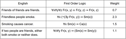
Understanding the data
There’s a lot to unpack here, especially for those unfamiliar with formal logic syntax. Firstly look at the first and last columns; we have natural language sentences and associated weights. The sentences denote relations and properties that should appear in generated data, and the weights denote how strongly these should be adhered too.
Larger weights mean that we should find examples in the data that agree with the sentences more often than lower weights. The weights can therefore be thought of as the unnormalised truthfulness of each of the sentences when applied to all data points. The weights are not probabilities as such but there should be some sensible way to map between the two.
The central column is a representation of the sentences using first order logic. Let’s break one down to get an idea of how the syntax works.
Here’s the first example:
∀x∀y∀z Fr(x, y) ∧ Fr(y, z) ⇒ Fr(x, z)
Variables
The letters x, y and z represent variables over which the expressions are evaluated. In this case, they refer to people from the group. The symbol ∀ denotes ‘for all’, so the meaning of the first part is fairly straight forward:
∀x∀y∀z : For all x, y, and z . Where x, y, and z denote individuals in the group.
Relations and combinations
The relation Fr(x, y) denotes a friendship relation between two individuals, and will return a truth value in the interval [0,1]. The symbol ∧ can be though of as a logical AND, known as the logical conjunction.
In Boolean logic this is simply that both of the inputs must be 1 for the output to the 1. But Boolean logic only works with 0s and 1s. In real logic it is slightly more involved as the operator needs to work for any pair of real numbers in the interval [0, 1]. Therefore conjunction is obtained via a t-norm operator such as min(x, y).
Putting this together we can obtain the meaning of the next bit of the expression:
Fr(x, y) ∧ Fr(y, z) : The truthfulness of two pairs of individuals being friends, where both pairs have a common person y.
Implications
Finally the ⇒ symbol denotes implies: so a ⇒ b means if a is true, then b is true.
Putting this all together, we can see how the full expression says:
∀x∀y∀z Fr(x, y) ∧ Fr(y, z) ⇒ Fr(x, z)
For all sets of three different individuals denoted x, y and z: if x and y are friends, and y and z are friends, then this implies that x and z are friends.
Which is summarised more concisely in the first column of the table.
Final elements
To understand the remaining expressions, the final syntactic elements are simply:
Sm(x): The truthfulness that an individual is a smoker.
Ca(x) : The truthfulness that an individual has cancer.
¬ : The logical NOT operator. In real logic this can be 1- the value for example.
∃y : There exists a y.
⇔ : Double implication, truthfulness of expressions on either side imply the other.
The authors of the paper showed that their approach to real logic allowed the knowledge base to be completed to a high accuracy, and that their implementation was able to predict relations and properties of individuals that are out of the reach of conventional first order logic systems. So how did they do it?
General Ideas
The overarching concept employed is to replace the elements of the first order logic systems:
Symbolic variables are represented by n-dimensional vectors.
Predicates, relations and functions are represented via matrix transformations.
x∧y : conjunction e.g. logical AND represented via t-norm e.g. min(x, y).
x∨y : disjunction e.g. logical OR represented via s-norm e.g. max(x, y).
¬x : negation e.g. logical NOT represented via functions e.g. (1-x).
Embedding
Symbols are embedded into a vector representation, similar to how words are embedded into vectors in deep learning systems for natural language processing. This could be for example a look up table containing entries for all legal symbols, mapping each of them to a vector of real numbers.
Transformations
If we wish to represent logical relations and functions with matrix transformations, then we cannot easily directly solve which matrices correspond to the desired function. Even the problem of how large a matrix needs to be to obtain the correct transformation is non-trivial.
The authors of the paper therefore define a method to assess how well a given matrix performs the task at hand, and claim that if we are able to solve the problem within a reasonable margin of error, then that is good enough. This is introduced via three concepts:
Satisfiability – this defines the error of a particular solution, it is said to be satisfied if the error falls within an acceptable margin.
Grounded theories – defines an arbitrary transformation applied to an arbitrary input set of variables, that maps to a real number in the interval [0, 1].
The satisfiability of grounded theories – a grounded theory is said to be satisfied when for all variables, the output of the transformations falls within the satisfiability region.
Deep neural networks
The authors then go on to say that if a grounded theory cannot be satisfied completely, then we are interested in finding the transformation that minimises the extent to which outputs fall outside of the satisfiable region.
This idea fits very closely with the concept of minimising a loss term in a deep learning system. We can imagine a candidate grounded theory (transformation) that is not satisfied, being iteratively optimised by backpropagation, using the extent to which it is not satisfied as a loss term.
Applications
We decided to extend the idea of LTNs to a new domain, computer vision. The rationale for this is that maybe by using such a formulation, we would be able to examine a computer vision system and ask it ‘questions’ by evaluating the truth of first order logic expressions. The end goal of which may be to end up with a system that can be examined using first order logic.
This may be of particular interest to people developing safety critical computer vision systems such as autonomous vehicles, as engineers would be able to assess why they failed, and essentially debug their complex systems using natural language.
Just like in the Smokers and Friends problem, we want to be able to present the system with incomplete information, and have it predict the missing elements. We can also use the output of the LTN modules to construct a full end-to-end network, where each module is explicitly constrained to, and guided by a humanly understandable concept.
An auxiliary benefit is that we can test the functionality of the LTN modules on out-of-distribution validation data that has not been seen during training, and look at which elements of the system fail first. Furthermore, when weaknesses in such a system are identified, they are insulated from the entire end-to-end model. This means that if we need to retrain a system module, then it will not cause catastrophic forgetting across the entire system.
In order to extend LTNs to a computer vision system, all we need to do is change the embedding function. Instead of using an arbitrary mapping defined in a look-up-table, we can use a transformation directly from the pixels. We could, for example, use a randomly initialised matrix to transform from the input symbols to a feature vector, or perhaps we can do better, and train a neural network.
This would then map an image to a vector that has an abstract semantic meaning, providing relevant information for other modules that rely on this vector as input. In this formulation, the input pixels are the ‘symbols’ and a convolutional neural network can be used to map the input symbols into an n-dimensional vector representation containing an abstract feature map. Once this vector is obtained then the whole LTN system can be constructed in the same way as in the Smokers and Friends example.
We created a toy problem involving traffic on a road. The road has three lanes, there are four ‘entities’: three vehicles and an obstruction. Vehicles are considered obstructed if there is an obstruction occupying the same lane. The distance to the obstruction was uniformly generated in a normalised interval between 0 and 1, where 0 denotes a vehicle right next to the obstruction and 1 a vehicle at maximum distance from the obstruction.
A crash would be resultant from the vehicles and obstructions on the road, if a given vehicle is within a critical distance from an obstruction in its lane. Each vehicle has a different critical distance at which a crash will happen. The goal was to create a framework of real logic that can detect crashes directly from an image.
The images were generated randomly according to the following probability distributions:
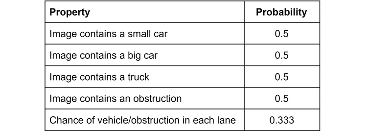
Here is an example of a randomly generated image.
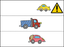
This image contains a ‘small car’ in the top lane, a truck in the central lane and a ‘big car’ in the bottom lane. We can see that the small car is obstructed, and the distance between the vehicle and the obstruction is small. In this image we would like to predict that a crash will happen, because the small car cannot avoid the obstruction.
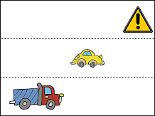
A crash is not present in the above image, because although there is an obstruction, it is not obstructing the path of any vehicle.
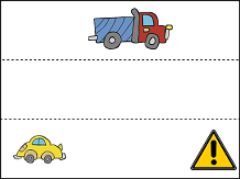
The above image also does not contain a situation where a crash will emerge because the distance of the yellow car from the obstruction is large enough that the car can manoeuvre to avoid a collision.
A crash will only happen if there is a vehicle and an obstruction in the same lane, within a pre-specified distance of each other. Each critical distance is different for each type of vehicle and unknown to the model, but is generated via the following rules:
A small car will crash if its distance to an obstruction in its lane is <~0.3.
A big car will crash if its distance to an obstruction in its lane is <~0.34.
A truck will crash if its distance to an obstruction in its lane is <~0.21.
These figures are based on the assumption that he vehicles travel at different speeds, and therefore take a different amount of distance to stop or change direction.
We wanted to create an LTN system that can predict crashes present directly from the image pixels. Unlike an end-to-end model, we can then take this LTN and use it to test the validity of logical hypotheses and see if they are what we would expect.
We can, for instance, test the validity of the hypothesis that a crash will happen if there is no obstruction present on the road:
¬Contains Obstruction(Image) ⇒ Crash(Image)
Each image was converted into an n-dimensional feature vector f using a convolutional neural network based encoding function.
Encoding(Image) → f: N-dimensional Feature Vector
We define a shorthand for this function for brevity in later expressions:
e(Im) → f:
Real logic functions were created to describe the contents of the image: the existence of entities, and whether the entities are obstructed, each of which take a feature vector as input, returning a truth value t in the interval [0, 1]:
Small Car Exists(f) → t: Truth Value ∊ [0, 1], shorthand: sce(f)
Big Car Exists(f) → t: Truth Value∊ [0, 1], shorthand: bce(f)
Truck Exists(f) → t: Truth Value ∊ [0, 1], shorthand: te(f)
Obstruction Exists(f) → t: Truth Value ∊ [0, 1], shorthand: oe(f)
Small Car Obstructed(f) → t: Truth Value ∊ [0, 1], shorthand: sco(f)
Big Car Obstructed(f) → t: Truth Value ∊ [0, 1], shorthand: bco(f)
Truck Obstructed(f) → t: Truth Value ∊ [0, 1], shorthand: to(f)
Further real logic functions were created to define the distance from each vehicle to an obstruction:
Small Car Obstruction Distance (f) → m: Magnitude ∊ [0, 1], shorthand: scd(f)
Big Car Obstruction Distance(f) → m: Magnitude ∊ [0, 1], shorthand: bcd(f)
Truck Obstruction Distance(f) → m: Magnitude ∊ [0, 1], shorthand: td(f)
Finally, a function was created that takes the above predicted quantities and returns a probability that a crash will happen.
Crash(t, t, t, t, t, t, t, m, m, m) → t: Truth Value∊ [0, 1]
The crash function, returning a truth value, operates directly on the outputs of the prior functions as follows:
For a given input image Im:
f = e(Im) : (We take the image and extract the feature vector)
Crash(sce(f), bce(f), te(f), oe(f), sco(f), bco(f), to(f), scd(f), bcd(f), td(f)) → t
We will abbreviate it to Crash() in future for brevity, but keep in mind it is always called with the above arguments.
The LTN architecture is summarised in the below image:
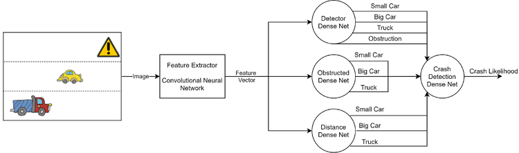
The randomly generated images were labelled according their content, such that each image in the training set had a complete description. There were 15000 total images divided into a training and validation set. We then trained several small neural networks based on these labels so that each network would represent one of the above functions.
A combined loss term was generated by summing the mean squared error of each model’s prediction (scaled by the number of relevant samples). This loss was also backpropagated into the embedding network in order to generate relevant feature maps from the input images. All models were trained in this way until the loss plateaued.
Each of the LTN modules were evaluated on a validation set that was entirely unlabelled. Similar to in the Smokers and Friends problem it was of interest to us to see if the real logic functions generalised to unseen validation data. As a first step, we evaluated the accuracy of each network returning a truth value, and looked at the average error of the networks trained to predict the distance of vehicles to an obstruction.
Validation Accuracy (%):
→ Small Car Detection: 98.83
→ Big Car Detection: 99.07
→ Truck Detection: 99.2
→ Obstruction Detection: 99.07
→ Small Car Obstruction: 98.8
→ Big Car Obstruction: 99.07
→ Truck Obstruction: 99.07
→ Crash Prediction: 98.63Average Distance Error (%): 5.37
As can be seen in the above performance data, each of the networks was trained to a high degree of accuracy when tested on the unseen validation set. This is great, and the end-to-end model is able to predict a situation that will lead to a crash with a high degree of accuracy. We can now closely examine how the system works by evaluating the truthfulness of different statements composed in first order logic.
Using the trained models, we were then able ask questions using first order logic.
Question 1:
What is the likelihood of a crash without a detected obstruction?
∀ Im ¬(oe(e(Im))) ⇒ Crash()
In order to assess the above expression it is a fairly simple process. We simply predict the crash likelihood of every image in the dataset and combine this using the t-norm (AND) operator of choice with the negated assessment of whether an obstruction exists in the image. We then average the values over every item in the validation set, and this gives us our model assessment as calculated on unseen data.
Answer:
∀ Im ¬(oe(e(Im))) ⇒ Crash() = 0.01
This is good! It shows that the system has almost no faith that a situation where there is no obstruction can lead to a crash, which reflects the rules of the road.
Question 2:
What is the likelihood of a crash when a vehicle is in the same lane as a detected obstruction?
∀ Im sco(e(Im)) ∨ bco(e(Im)) ∨ to(e(Im)) ⇒ Crash()
This question was evaluated similarly to Q1 with the inclusion of the s-norm operator (OR).
Answer:
∀ Im sco(e(Im)) ∨ bco(e(Im)) ∨ to(e(Im)) ⇒ Crash() = 0.26
This shows that the model has learned that where a vehicle is in the same lane as an obstruction, it is somewhat likely that there will be a collision, however the likelihood is fairly low.
This is because the randomly initialised distance between the vehicles and obstructions is usually large enough such that no collision will happen. This again shows that the model has learned something useful and can apply it to unseen data with confidence.
Question 3:
What is the likelihood of a crash when a vehicle is in the same lane as a detected obstruction, and where the distance is below a certain threshold between 0 and 1?
∀ t∊ [0,1]∀ Im (sco(e(Im)) ∧ (scd(e(Im)) < t)) ∨ (bco(e(Im)) ∧ (bcd(e(Im)) < t)) ∨ (to(e(Im)) ∧ (td(e(Im)) < t)) ⇒ Crash()
For this assessment we calculated the probability in the same way as before, however we varied the threshold variable t and graphed the result:
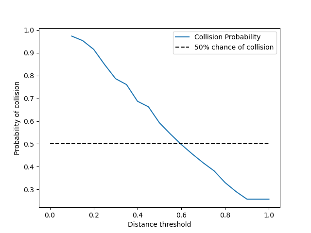
As can be seen in the graph, on average, when the distance threshold is under around 0.6 there is an above 50% chance of collision, which makes sense if we remember that the average threshold for all vehicles to collide was around 0.3 and the distance is uniformly distributed.
Question 4:
What is the likelihood of a crash when a truck is in the same lane as a detected obstruction, and where the distance is below a certain threshold between 0 and 1?
∀ t∊ [0,1]∀ Im to(e(Im)) ∧ (td(e(Im)) < t) ⇒ Crash()
We did the same procedure as in Q3, but this time we were only interested in trucks.
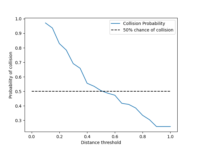
In this graph the distance threshold at which there is a greater than 50% chance of collision is lower (around 0.5), this shows that the model has learned that trucks travel slower than the other vehicles, and therefore need to be closer to obstructions to result in a collision. It has learned this directly from the data and it has been evaluated on unseen data, directly from pixels.
We have shown how logic tensor networks are able to combine concepts from formal logic and deep learning. Advantages of this approach include an ability to make inferences that go beyond traditional first order logic systems. Furthermore, this approach allows us to look under the hood at our deep learning models, and use first order logic to evaluate how they work.
This technique has the potential to allow greater model transparency and explainability. Increased insight into how models work could lead to greater public confidence in safety critical systems, and allow for engineers to detect and remove blind spots in models when applied to unseen, out of distribution data.
• • •
At Optalysys, we have developed an optical processor that is able to calculate convolutions far more efficiently than what digital electronics can achieve. We have demonstrated the utility of this approach in this paper. We can therefore use our hardware as a platform to run neurosymbolic AI systems at state of the art efficiencies. Autonomous vehicles powered by Optalysys optical processing technology will be able to go further, more safely and with a lower carbon footprint than any electronic hardware system.
News
© 2023 All rights reserved Optalysys Ltd
Subscribe
Sign up with your email address to receive news and updates from Optalysys.