
Optalysys: What we do and why we do it
In this article, we give an overview of what our optical system is, how it works, and why it’s so useful. This is what we do, and why we do it.
Since the early days of the silicon revolution, the course of processor development has followed a spectacular yet predictable arc. This prediction, the promise that the chips of tomorrow will be vastly more powerful than the ones of today, has for the last 50 years been encapsulated by Moore’s law, the observation that the density of transistors on a chip doubles roughly every two years. This persistent and reliable exponential growth in computational power has fuelled staggering global change and a correspondingly vast market for computing hardware. However, the promise of tomorrow is no longer the same…
Conventional computing is rapidly approaching the physical limits of what can be achieved with silicon electronics. As the size of the transistors used by electronic processors to create complex logic-solving circuits continues to shrink, gains in performance are becoming outweighed by growing electrical power consumption and thermal management requirements.
Moore’s law is now beginning to break down in the face of these fundamental performance limits.
The breakdown of Moore’s law coincides with an unprecedented explosion in demand for processing power. As the reach of the digital world begins to extend into most areas of modern life, the need to extract insight from the vast quantities of data produced by an ever-growing network of devices and applications has led to the era of machine learning. Rising to meet this demand, huge advances have been made in the development and use of Graphics Processing Units (GPUs) and other specialist processors which can perform these tasks with far greater speeds and efficiencies than a Central Processing Unit (CPU). However, these co-processors still face the same fundamental limitations of every other electronic system.
As a result, there has been a push towards radically different types of information processing using alternatives to silicon electronics. Quantum computing is a prime example, as are biologically-inspired systems that take their inspiration from the function of the brain (so-called “Neuromorphic” systems) or indeed from even more exotic sources.
Performing calculations using light, optical computing, is one of these processing solutions. At Optalysys, we have developed a unique optical computing system to bring incredible processing power and energy efficiency to everything from data-centres to edge computing.
What Is Optical Computing?
Light has some remarkable properties. Famously, it acts as both a particle and a wave. Individual photons are discrete packets or “quanta” of energy, but they have no mass and travel as an oscillation of the electromagnetic field. This wave-like property allows a beam of light to interfere with itself, the waves either cancelling or reinforcing each other in different locations, creating “interference fringes”.
This effect can only usually be seen under certain conditions. The light has to be initially coherent, which means that all the photons start out sharing the same frequency and a consistent phase relationship. This is the kind of light produced by a laser. If the phase of any part of the light is altered, the interference pattern changes.
It is this ability of light to interfere with itself that forms the basis of computing with silicon photonics. By manipulating these properties so that we can represent and store information in beams of light and then allow them to interact, we can perform a calculation without using any transistors at all, thus overcoming the limitations of Moore’s law.
The rise of artificial intelligence and machine learning techniques has spurred efforts across the computing world to make these tools work faster. A significant part of executing most machine learning models is performing multiplication operations on what are known as “matrices”, grids of numbers that have specific mathematical rules for (amongst other things) multiplication and addition. In a hardware context, these multiplications can be performed using elementary “Multiply and Accumulate” (MAC) operations.
While the operations needed for machine learning are almost entirely multiplications and additions of two numbers, a great many of them need to be performed in a very short period of time. Graphics Processor Units (GPUs) and even more specialised Tensor Processing Units (TPUs) are the fastest way of performing these tasks using silicon electronics.
The optical alternative, silicon photonics, offers an entirely different way of performing these operations at incredible speed, and most companies working in silicon photonics are pursuing a similar objective to this.
Optalysys are taking a different approach. Simple multiplication is not the only useful computing process that can be accelerated by silicon photonics, and our hardware is designed to perform another very specific mathematical function. This function is not only of tremendous importance to scientists and engineers, but has great relevance to the digital world around us.
If you’ve ever watched a show on Netflix, listened to a piece of digital music or just browsed the web, this function has been applied countless times in analysing, processing, and transmitting this information.
This function is known as the Fourier Transform.
The Fourier Transform
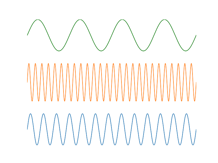
The Fourier transform is a mathematical tool for analysing repeating patterns. Given a piece of information, which could be an audio track, an image, or a machine-learning data-set, the Fourier transform gives a way by which we can unpick and isolate the simple wave-like harmonic patterns (sines and cosines) that, when added back together, return the original piece of information.

For such a phenomenally powerful tool, it has a surprisingly simple equation:

Despite the deceptive simplicity, this mathematical function has applications across the entire spectrum of information and data processing. In some cases, the Fourier transform is directly useful, such as when we are dealing with signals that contain information that we want to extract or alter. In other cases, it can massively simplify complex problems that would otherwise be intractable. To say that it is one of the most useful mathematical functions in history is not an overstatement.
However, when we want to apply the Fourier transform using a computer, there’s a catch. The most efficient computational method for performing a Fourier transform on a data-set, the Cooley-Tukey Fast-Fourier Transform (FFT) algorithm, has to break the data-set down into many smaller Fourier transforms and then progressively recombine them. This need to perform multiple operations, one after the other, means that there is a fundamental limit to how efficiently a digital system can perform the Fourier transform.
Digital Efficiency of the FFT
If we want to use the Fourier transform to simplify a problem or speed up a calculation, we have to contend with this problem of efficiency.
In computer science, the measure of algorithmic complexity is often written in what is known as “Big-O” notation, which gives us an idea of the minimum number of operations that need to be performed when running an algorithm. For example, if we need to perform n operations given n pieces of data, this is an “O(n)” algorithm with linear complexity. If instead we need to perform n² operations, we’d say that the algorithm works or “scales” in polynomial time. Here’s what that looks like on a graph.
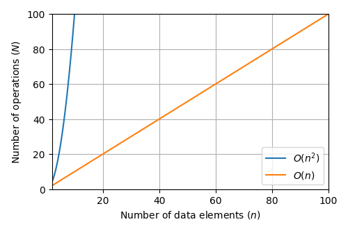
As we can see, n² becomes computationally “expensive” very quickly! This scaling is important, as a single computer processor core can only perform one operation at a time. Because the system “clock” that governs the rate of operations has a maximum speed (usually about 3.5–4 GHz on a modern desktop CPU), an increase in the number of operations needed to carry out a task means a direct increase in the amount of time it takes to complete that task.
For n pieces of data, the FFT algorithm must perform at least O(n log(n)) operations. For reference, here’s what O(n log(n)) looks like on a graph, compared to an O(n) operation.
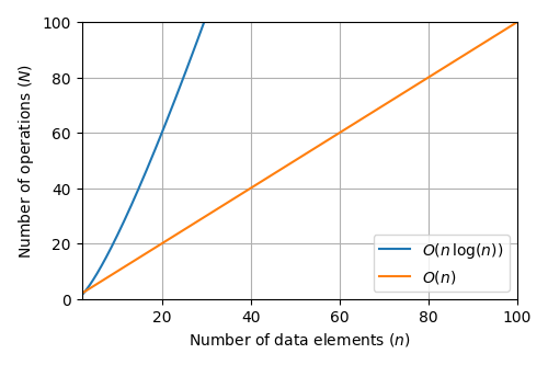
That’s still pretty expensive! It’s an open question in computer science if this O(n log (n)) scaling is a fundamental bound on the efficiency of the digital Fourier transform, but the technology Optalysys has developed finds a way around this.
Fourier Optics
The interference patterns produced by light reveal something fundamental and deeply beautiful about the universe, but they also have useful properties. Under specific circumstances, if we focus the interference patterns created by a light source that contains light of different phases and intensities, the pattern of intensity and phase that we see at the focal plane corresponds to the Fourier transform of the original light source. For our purposes, this means that light can perform the Fourier transform instantly, in O(1) time!
Here’s what O(1) time looks like when compared against O(n) and O(n log (n))
O(1) time is the green line at the bottom. It’s flat, because the number of operations doesn’t increase as we add more data to the calculation. This is what makes the Fourier-optical approach so powerful; not only does it return the answer instantly, it does so regardless of the amount of information put into the optical system!
The way that light from the source spreads out and interferes with itself is doing the work for us in a massively parallel calculation, without a single bit of the Fourier transform having to be done in electronics.
Aside from shattering the theoretical limit for the digital Fourier transform, the inherent light-speed processing of the optical method means that this is likely the fastest possible method of calculating the Fourier transform. In a single technological leap, the limitations of the Fourier transform have moved away from the number of operations that must be performed, to the speed at which information can be fed into the system.
Not only does this represent an enormous increase in processing power, but this method of calculation is tremendously energy efficient compared to conventional electronic systems. Besides the inherent efficiency of not having to use transistors, the optical process also doesn’t generate any excess heat, so there is much less need for power-hungry cooling solutions.
Fourier optics itself isn’t a new technology itself, and Fourier optical systems have been used for basic pattern recognition purposes since the 1960s. But using Fourier optics to process any data we want, using optics as a general-purpose information processor, means finding a way of writing that information into the light, a much more difficult and complex task.
Previous implementations of this type of system were based on liquid crystal micro-displays that encoded information into the laser light, using bulk optical components and discrete camera sensors.
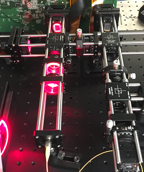
However, aligning the laser and lenses correctly is a difficult task, and the entire system is so sensitive to movement it has to be assembled on a special vibration-isolating optics bench.
Optalysys’s previous developments have produced optical co-processor versions of such systems mounted to drive electronics that can be installed into PC motherboards.
These systems had very high resolution in the millions of pixels. This might seem useful, but the use of liquid crystal displays also made them very slow, with speeds in the kHz range at most. Furthermore, many tasks for which the Fourier transform is most useful (such as in deep learning) don’t benefit from very high levels of resolution.
Instead, by using the light-transmitting properties of silicon, we can build optical circuits directly into a micro-scale system, eliminating the problem of size and vibration while working at a resolution which is useful for many more tasks.
This is what Optalysys have now done; we took our expertise in computing and optical systems, and used it to design an integrated silicon photonic processor to perform the Fourier transform at a speed and power consumption that was previously impossible.
And then, once we were done designing that system, we made it a reality.
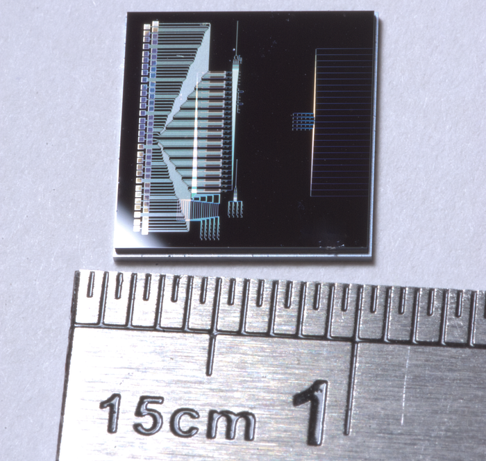
This is the world’s first silicon-photonic system for general Fourier-optical computing. Not only does the dramatic reduction in size mean that the benefits of this kind of computing can be part of many more applications, but the switch to silicon photonics allows us to use faster components for controlling the light.
Because these components can operate at speeds well beyond those of conventional electronic integrated circuits, when coupled with the phenomenal speed and scaling of the optical Fourier transform, this yields the potential for truly unprecedented calculation throughput. This architecture allows us to perform a Multiply-and-Fourier Transform operation, or MFT, at incredible speed.
Now, applications and uses of the Fourier transform that were previously locked away by computational effort and power consumption are made possible. A new era of fast computing with light, powered by our technology, is dawning.
As we continue with our development, we’ll be using this space to explore the underlying scientific and technological uses of this system across a vast array of tasks that extend from cutting-edge research through to the end-user. Our next articles on Medium, coming soon, will explore the use of our system in applications as diverse as cryptography, artificial intelligence, and computational fluid dynamics.
At the same time, we’ll be talking about how optical systems can effectively work alongside conventional electronics, and showcasing the engineering that makes this possible.