
If you’ve been reading our previous articles in this series about the workings of our optical computing system, we’ve been talking about how we can use our technology to set up an optical field that carries numerical information, and then process that optical field with a lens in order to calculate the Fourier transform of that data. In this third article we’ll be talking about the last stage of that process, in which we extract the relevant information from the optical field after processing and convert it back into a form that can be understood and managed by a digital computer.
To do so, we’ll first need to show that the real and imaginary components of the Fourier transform are present in the output field. Next, we’ll talk about how we can detect these components simultaneously. Along the way, we’ll be comparing predictions to real data from calculations performed on our prototype system.
In our last article, we examined the free-space optical stage of our system. This is the arrangement of passive optical elements such as prisms and lenses through which light emitted from the silicon photonic section can interact and interfere and in the process calculate the Fourier transform of the data represented in the optical field.
The light that reaches the detection plane is just that; light. Its passage through free space and the lens has altered the pattern of the wave front but it is still a physical thing, a very particular arrangement of the electromagnetic field. To make use of it as the output of a calculation we must first quantise it, turning the measurable properties of this field into a digital representation.
In the final system, the second micro-lens array focuses the field onto a second array of grating couplers which send the light back into a silicon photonic circuit, allowing us to analyse the properties of the field using on-chip components.
The quantity measured by the photodetectors represents the squared absolute value of a Fourier transform, rather than the Fourier transform itself. For many applications, it is important to know the full complex Fourier transform. Fortunately, we can recover the data we want from its absolute value. The way we perform this calculation here is only illustrative of the fact that this information is present in the optical field; we’ll get on to the way this works in the final system in a bit.
The following relies on the fact that the two operations done by the MFT unit, multiplication by complex numbers and the Fourier transform (and their combination) are both linear. Let us call F the combination of the two operations. Linearity means that, if X and Y are two possible inputs (vectors in the one-dimensional case or matrices in two dimensions) and a is a complex number, then
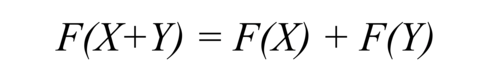
and

These two equations can be used to show that, for any vectors or matrices X and Y of complex numbers,

where a star denotes complex conjugation and ‘Re’ denotes the real part of a complex number, and

where ‘Im’ denotes the imaginary part. In both equations, you can see that the term on the left-hand side of the equals sign is the squared magnitude of the Fourier transform of X + Y. This is the field that arrives at the detection plane. The terms on the right hand side show how this can be broken down into a linear combination of distinctly different parts. All the multiplications and additions are all done component-wise, where individual elements of X and Y are added or multiplied together.
Let us assume that we know F(Y); for instance, that it is easy to compute or has previously been computed, and that none of its coefficients vanish. Then, F(X) can be computed using the formula

Looking at the terms on the right-hand side, we can see terms that represent the squared absolute values of F(X), F(X+Y), and F(X+iY). These can all be calculated by using our system three times to directly find the squared absolute Fourier transform of X, X+Y, and X+iY.
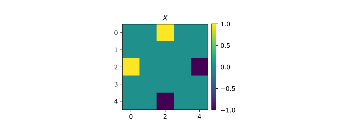
We can show how this works with a specific example. Let us consider a device with a 5 by 5 input performing a simple discrete Fourier transform, i.e., with the phases set to 0 for each multiplication unit. We choose Y as an array with coefficient of index (0,0) equal to 1 and all the others equal to 0. Its Fourier transform F(Y) is then the 5 by 5 matrix with all its coefficients equal to 1.
Let us consider the following example input, denoted by X in the following:
We would like to compute its Fourier transform using an MFT unit. To this end, we first use the MFT three times with inputs X, X+Y, and X+iY. The corresponding three outputs are shown below (results from numerical simulations):
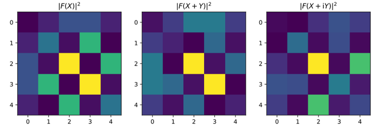
We can then combine these three outputs to find F(X) using the above formula. Here are the results for the real part of the Fourier transform:
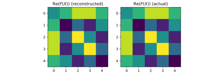
As we can see here, the ‘reconstructed’ result obtained using the three simulated outputs from the MFT returns the real part of the actual Fourier transform. Let us do the same for the imaginary part:
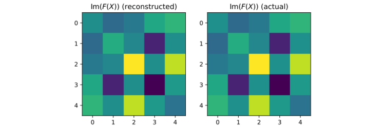
Again, the actual and reconstructed results match exactly. While we verify this result here for only one specific case, this holds for any possible input, real or complex.
We now show some experimental results obtained from our optical device. At the current state of development, we are using a 5 by 5 array of pixels for the input and output. These numbers will be increased in the near future, but this demonstrates that the optical Fourier transform can be performed with our system.
The three plots below show the squared absolute value of the Fourier transforms of different inputs. This quantity is proportional to the light intensity and can thus directly be ‘seen’ using a camera or photodetectors.
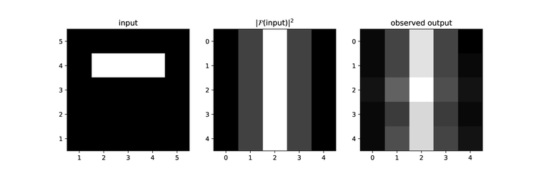
Results for an input with three pixels equal to 1 (white pixels in the left panel) and the others set to 0 (black pixels in the left panel). The middle panel shows the squared absolute value of the Fourier transform, computed using a Python script and the NumPy library. The right panel shows the light intensity measured from the optical device.
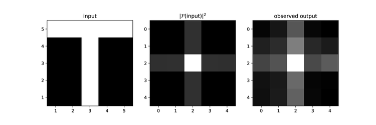
Results for an input forming the letter T. As in the previous figure, each pixel of the input is set to 0 (black) or 1 (white); the middle panel shows the simulated output and the right panel shows the observed light intensity from the optical device.
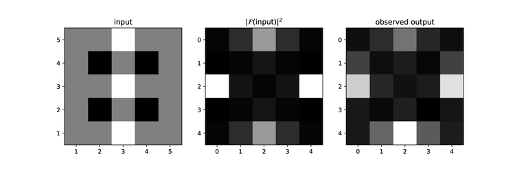
Results for an input with pixels set to -1 (black), 0 (gray), or 1 (white).
We can see that the observed outputs, the images we see when we look at the Fourier plane of our system with a camera, are very close to the digitally calculated values.
To quantify the difference more precisely, we can compute the root mean square error (preliminary results returned an error of ~10%).
But we want to go further and compute the full complex Fourier transform to confirm this. To this end, we can use the technique outlined above. Results for four different inputs are shown below:
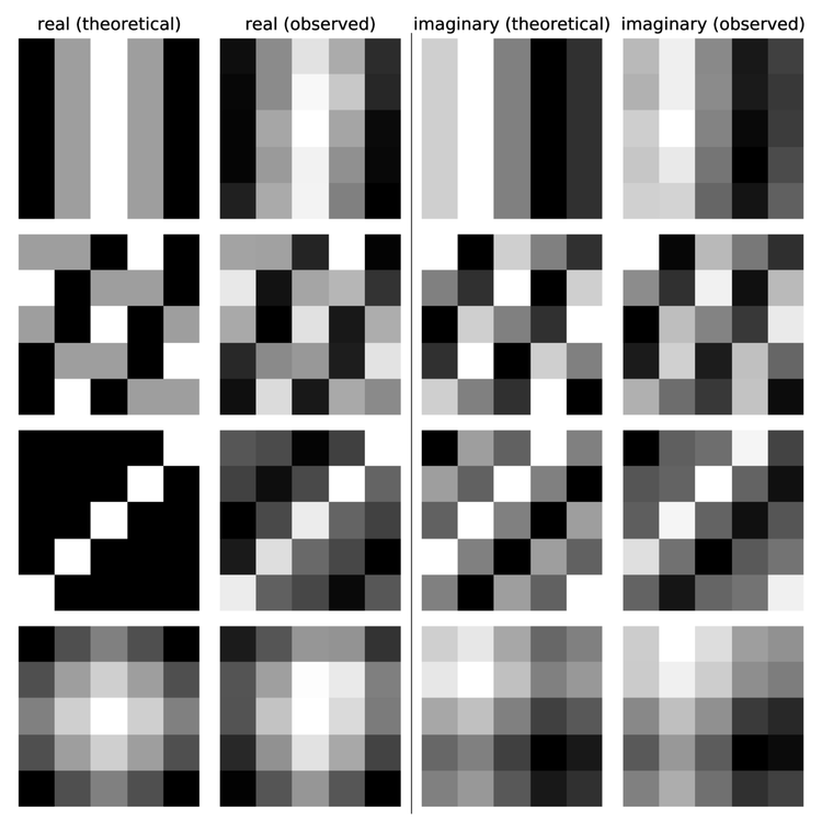
Complex Fourier transform for four different inputs. The first and third columns show the simulated real and imaginary parts, respectively. The second and last columns are experimental results.
As for the plots of the intensity, the observed results are close to the theoretical ones — again, the root mean square error is of the order of 10%.
The images we show above were captured with an infra-red camera looking directly at the output plane of our system. This allows us to make tweaks and changes, but it isn’t the way in which the final system will work.
In our final system, we replace the camera with an array of balanced photodiodes. This allows us to recover both the real and imaginary components simultaneously, in a single optical frame.

A balanced photodiode array. When each diode outputs an equal current, the total current is zero. By exposing one diode to the original optical source and the second to the output of the optical Fourier transform, we can compare the relative phase and extract the complex value output.
The set of two balanced photodiodes allow us to compare our original light source with the detected optical calculation in order to work out the relative phase difference and thus determine the complex output. The transinductance amplifier converts the output current to a voltage which can be processed by an analogue to digital convertor, which quantises the signal into discrete digital bits. Once in this form, the information can be used in other calculations in a conventional digital computer.
This completes the optical Multiply and Fourier-Transform (MFT) process, and with it this series of articles describing our core technology. There is of course much more to this particular method of optical computing; from our choice of optical modulators and supporting electronics that will allow us to take advantage of the spectacular bandwidth of optical systems, through to the calibration techniques required to manufacture systems on a large scale, Optalysys continues to push ahead with the development required for commercialisation.
News
© 2024 All rights reserved Optalysys Ltd
Subscribe
Sign up with your email address to receive news and updates from Optalysys.