
Modern CFD techniques give us impressive capabilities when it comes to designing things like safer aircraft, more efficient wind turbines and better streamlined cars, but they also come at an incredibly high cost in money, time and energy. This is because we have to repeatedly solve vast numbers of equations representing small changes in flow properties over time. We asked if there was a better way of doing this.
There is.
In our last article, we gave a brief introduction to the field of computational fluid dynamics (CFD) and described one of the most popular methods for solving fluid flow problems.
In this approach, the fundamental Navier-Stokes equations that describe the behaviour of fluids are first converted into a form which is compatible with digital calculation methods, creating a set of transport equations for the various different fluid properties (mass, momentum and energy).
By breaking up the region of fluid flow that we are interested in into many smaller individual volumes and then calculating the transport of fluid properties between them, we can find solutions to problems in fluid dynamics which would otherwise be totally impractical to work out by hand. This approach is the most common methodology in the field, but it is by no means the only one.
In this article, we look at how techniques from deep learning can be applied to fluid dynamics in a way that upends some of the most fundamental limitations of current techniques, potentially slashing the financial and computational cost to a fraction of what it was while making the benefits of CFD more openly available to non-specialists. Along the way, we demonstrate the application of our optical computing system in performing the core mathematical operations for both old and new approaches to CFD.
This is a long article, so we’ve structured what we found into two distinct sections. In the first section, we describe how we generate flow fields that we can solve using an existing method in fluid dynamics which can also be applied using optical technology. We can then use these fields and their solutions to train a deep learning network.
In the second section, we use the data from the conventional method to demonstrate the effects of kernel size on network training. We then show how a “super-resolution” neural network can be used to reconstruct a higher resolution solution from low resolution data, and use our optical system to perform this task.
This combination of a highly efficient method of computing paired with revolutionary simulation techniques offers a future in which CFD is not only commonplace and accessible but wildly more efficient. Let’s get started.
Testing out an AI approach means that we need a large quantity of relevant training data. This means that we need a way of quickly generating and solving many fluid flows involving similar phenomena. As vorticity is a major component of many flows, we decided to hit two targets at once; we’re not only going to generate training data, but we’ll do so using a conventional CFD method which could also be solved using optical technology.
Everything in this section is solved using conventional electronics because we want to be able to use it to test out a deep learning network that uses our optics. That means we need to be able to make comparisons to the electronic solution, but it’s worth keeping in mind that the technique we previously described for performing large Fourier transforms using a Fourier optical processor can also be applied here, with all of the associated benefits for power consumption and speed.
In our last article, we described the fundamental equations of fluid motion, the Navier-Stokes equations. The Navier-Stokes equations are a set of partial differential equations (PDEs) in which mathematical objects called operatorsact on parameters of the flow. Currently, the dominant method of calculating fluid flow involves dividing the flow region into thousands or even millions of smaller volumes known as a mesh.
In this “finite-volume” approach, the Navier-Stokes equations are then used to construct a set of transport equations which can be used to calculate the movement of fluid properties between cells. By repeatedly solving these transport equations over small time periods, we can get a numerical approximation to the behaviour of the flow.
There are many different ways of expressing the Navier-Stokes equations, depending on the flow configuration and on the various assumptions we can make to simplify the problem. In order to demonstrate how optical neural networks can be used to solve these equations, we focus on a comparatively simple formulation which exhibits many of the important properties of more general setups. The first simplification we make is to assume the flow is incompressible, which means that it has the same density at every point in the flow. The second is to reduce the number of dimensions of the problem, from the usual three spatial dimensions to two. The Navier-Stokes equations may then be written as:

We’ll briefly explain the meaning of each symbol used in this set of equations:
The boldface letter u represents the velocity field of the flow. It is a vector with two real components, which determines the direction and speed of the fluid at each point.
The letter w represents the vorticity of the flow. Roughly speaking, it tells us how fast the fluid is rotating: it will typically be large close to the centre of a vortex, for instance, and vanishes for a uniform flow. Its sign indicates whether the flow rotates anticlockwise (for positive values of w) or clockwise (for negative values of w).¹
The symbol ∂ₜ denotes the partial derivative with respect to time, yielding how fast a quantity is changing.
The symbol ∇ is the vector of partial derivatives in the two space dimensions.
The Greek letter ν denotes the viscosity of the fluid.
The letter f denotes a function used as a forcing term. Physically, it represents external forces (such as gravity) that contribute to fluid rotation.
Finally, the symbols · and ×respectively represent the dot product and vector product.
This system of equations determines how the velocity field and vorticity of the flow evolve in time starting from some initial condition. To be complete, we also need to consider the boundary conditions, which determine the behaviour of the vorticity w at the edge of the simulation. For simplicity, we used periodic boundary conditions. This are equivalent to assuming that the flow repeats itself periodically. Mathematically, for each x between 0 and 1, they may be written as:

and, for each y between 0 and 1,
We also impose a similar condition on the derivatives of w.
To solve the Navier-Stokes equation numerically, we discretise the space and time coordinates so that the total amount of information is finite. This approach is used widely in conventional CFD techniques based on Eulerian meshes. Given the configuration at a time t and the boundary conditions, the Navier-Stokes equations are used to determine the configuration at the next time coordinate t + δt, where δt is the time step. The solution to the Navier-Stokes equations over this time period is then used to calculate the next time-step, and so on.
Although the first line of the Navier-Stokes system we are working with is the longest of the three, it turns out to be straightforward to deal with. Indeed, it may be rewritten as:

If w and u are known at time t, then ∂ₜw can be calculated by evaluating the right-hand side and then used to acquire an approximation of w at time t + δt using the formula w(t + δt) ≈w(t) + δt ∂ₜw(t). Of course, more intricate numerical schemes can be used to get better approximations. Here, we will use this simple expression to make the numerical resolution straightforward, as our overall focus is on estimating the ability of neural networks to learn the solution, not on optimizing the standard approach. The complexity of this operation is linear in the number of points in the spatial grid: if the grid has N points, the number of elementary operations (additions, subtractions, and multiplications) needed to compute the solution at time t + δt from the solution at time t scales in O(N) for large values of N.
The next two lines, however, have no such straightforward resolution method. To our knowledge, the simplest and most efficient way to solve them is to perform the calculation in Fourier space. Fourier transforms have extensive utility in CFD; the large-eddy simulation method we briefly described in the last article is dependent on the ability to perform a Fourier transform as part of filtering out the smaller turbulent eddies. However, in this case, we’re applying a more general technique known as a spectral method for solving the Navier-Stokes equations.
Spectral methods are fundamentally different to the methods of solving fluid dynamics that we describe both above and in our last article, and the reason we haven’t focused on them until now is that they have a relatively limited range of utility. Rather than constructing and solving transport equations on a local level, spectral methods solve the fundamental differential equations by treating the entire flow domain as a sum of sinusoidal basis functions of different frequency. Substituting these basis functions into the partial differential equations described by the Navier-Stokes equations yields a set of ordinary differential equations which are easier to solve numerically. By contrast, as finite volume methods deal with a huge number of local solutions to the Navier-Stokes equations, they require more computation overall.
Spectral methods have some significant advantages with respect to numerical accuracy and speed, but this comes at the cost of major difficulties when it comes to certain problems. For starters, spectral methods don’t deal as well with the kind of variation in flow behaviour due to wall boundaries, the kind that you find in most engineering problems (hence our choice of periodic boundary conditions). Secondly, they can’t deal with flows containing discontinuities such as shockwaves. However, when it comes to fluid problems without boundary conditions (which do exist; global weather prediction is a good example, as there are no boundaries on a sphere!) or with simple ones (such as Dirichlet boundary conditions on a straight wall), spectral methods allow us to do things with a level of accuracy and efficiency that we simply couldn’t achieve using the finite element method.
Let’s continue. Denoting with a symbol ‘~’ the Fourier transform in the two space coordinates, these equations may be written as:

where k denotes the wave vector. Denoting the two components of each vector by an index x or y, these equations may be rewritten (after a few lines of algebra) as:

The field velocity u can thus be determined (up to a constant term, which would correspond to k = 0 ²) by performing a Fourier transform of w, using the above equations to get the Fourier transform of u, and then two inverse Fourier transforms to get the two components of u. When performed on a CPU or GPU, this sequence of operations has at best a complexity of O(N logN), where N is the number of points in the grid.
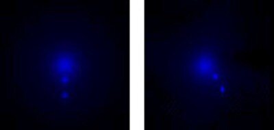
We create starting conditions for a vortex flow problem by generating random gaussian functions of a consistent amplitude, adding them together, and then using the resulting spatial distribution of values as our starting vorticity. We then solve the evolution of the flow using a spectral solution method.
The images below show an example of a vortex flow generated and solved in this way on a 64 by 64 grid. We choose a small grid for our solutions to reduce the time needed to train a neural network to learn the solution. The vorticity is represented by the intensity of the blue colour. The initial configuration (left) has one “large“ vortex at the centre and two “small” ones aligned vertically. At a later time, the two “small” vortices have rotated around the “large” one with a nearly constant angular velocity.
Here, we’ll take a brief moment to explore the impact of optical computing on spectral methods, which as discussed are essentially an application of the Fourier transform. The “easiest” algorithm for computing a Fourier transform (or its inverse) has a quadratic complexity in the size of the input: taking the Fourier transform of an image with N pixels requires a number of operations scaling as O(N²). A more efficient algorithm, the Cooley-Tukey fast Fourier transform (FFT), reduces the complexity to O(N log N)— a significant improvement, but this can still represent a computational bottleneck.
The optical Fourier transform, on the other hand, has a complexity in O(1): the runtime is the same regardless of the size of the input. Of course, in practice, the throughput is limited by how fast one can pass data to and read it from the system — but the Fourier transform bottleneck is completely eliminated! Even if we need to calculate a Fourier transform for a grid which is larger than the resolution of our optical system, we’ve previously demonstrated that the complexity overhead this introduces is still better than electronic techniques, scaling as:

For this reason, the optical device we are developing can reduce the runtime and energy cost of algorithms relying on the Fourier transform by several orders of magnitude.
Spectral methods for solving the Navier-Stokes equations could therefore be significantly accelerated using the Optalysys Fourier engine. However, if the time step is small, solving the equation could still take some time. Indeed, the number of time steps needed to evolve the configuration is proportional to the inverse of δt. Since this needs to be small for the numerical solution to be accurate (typically, the magnitude of the errors will be proportional to some power of δt), this number can easily become large.
That’s the end of the first section. We’ve shown how we generate fluid flows that can be solved using an optical hardware method using an existing and well-established technique. Now we’re going to take this method and apply it to something completely new: fluid-solving AI
Formally, the Navier-Stokes equations are a set of partial differential equations (PDEs) in which mathematical objects called operators act on parameters of the flow. As we’ve described above, we can use these equations as a starting point for a range of different techniques in order to get a numerical approximation to the behaviour of the flow.
Before moving on to the alternatives to this method, it’s worth considering what it is that operators in PDEs actually do. Physicists and engineers tend to view these things in terms of their physical interpretation, but the theory behind PDEs extends deep into pure mathematics.
One way of viewing PDEs is as a mapping between function spaces. A function representing, for instance, the configuration of a fluid at a given time, is mapped to another function representing its evolution at subsequent times.
However, a very recent advance in the field suggests that deep neural networks can perform a task called operator learning. In this approach, rather than starting with the rigorous mathematics of operators and creating a specific system of digital algorithms, the idea is instead to allow a network to learn the association between flow properties and outcomes directly from observations. It is this approach that we’re going to explore in the rest of this article. We’ll explain the benefits along the way.
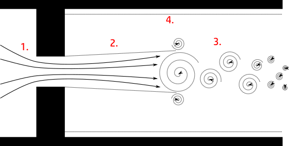
One of the major challenges with existing CFD solutions is the fact that fluid behaviour can vary significantly over a simulated region of interest. Consider a pipe with a small obstruction; the flow of fluid at the pipe wall will usually be laminar, the flow through the barrier will be heavily influenced by the presence of boundaries, while the flow downstream of the obstruction might include jet-spreading and turbulent behaviours which are better captured with different models. All of these different behaviours can exist in close proximity to one another within the same region of interest, which poses a problem when it comes to incorporating the relevant models into a single simulation. This localised variation in most problems is one of the shortcomings of the spectral method approach, which has to consider the whole flow domain at once.
Modern CFD packages are usually designed to simplify these challenges, allowing users to focus on the engineering rather than wrestling with model parameters in the software. Nevertheless, creating a useful and accurate CFD simulation still requires a lot of skill and awareness of these limitations.
By contrast, the significant benefit of operator learning is that there are no separate models that must be combined; instead a single network seamlessly blends all of these different behaviours together. Not only would an operator learning approach be potentially faster and more accurate, but it would require much less domain specific knowledge, allowing non-specialists to create and benefit from highly accurate CFD simulations. In a future in which this technique is commonplace, a user would simply define the working fluid, the flow region and the starting conditions, and then select a later time for which they would like to know the state of the flow.
Furthermore, deep learning based methods have been shown to be 3 orders of magnitude less expensive on standard electronic hardware. And with optical computing, we can take this already efficient technique and improve upon it drastically. Optical computing is well established as a highly competitive alternative to conventional electronics for deep learning tasks, and this application is no exception.
We’re exploring a deep learning approach based around convolutional neural networks which has previously been demonstrated by researchers from Caltech and Purdue University and Google Research. It makes use of the speed-up provided by the optical Fourier transform but does not require as many time steps. As we described above, the general idea is to use a neural network trained to learn the evolution from the initial configuration to the final one.
First, we generated 10,000 solutions of the Navier-Stokes equation using the same technique as applied for the spectral method. The neural network was then trained on these solutions, after which it was able to predict the evolution of a flow configuration even over a time period 100 times greater than the time-step used in the spectral approach! The results for the error between the machine-learning and spectral methods as a function of the number training epochs is presented in the following section, in which we examine the impact of filter size on the accuracy of the network.
In our last article, we identified the need to perform time-steps as one of the biggest reasons for the enormous cost of CFD. Timestepping means that the bulk of the calculations we perform are actively wasted, as we rarely want all or even most of the data from a simulation. This ability to step forwards over much greater time periods allows us to cut out the time and expense of this technique.
News
© 2024 All rights reserved Optalysys Ltd
Subscribe
Sign up with your email address to receive news and updates from Optalysys.