Scaling up: Using Fourier Optics for Bigger Transforms
The Fourier transform is a phenomenally useful mathematical tool applied throughout the scientific world.
Wherever nature contains a repeating pattern, the Fourier transform can be used to break that pattern down, converting the information into a form which is much easier to work with.
However, some of these patterns are quite large, and only fully reveal themselves over many data points. The optical method of computing the Fourier transform is extremely fast, but such systems will always have some physical limits to the number of data points they can work with at once. Light is a continuous medium but the individual components in our system that emit and detect light for processing are discrete and finite in number, so we’re faced with a very important question; can we perform a Fourier transform on a bigger array than the maximum resolution of a Fourier-optical computing device?
In this article, we’ll explain how not only is this possible, but how the optical method is fundamentally faster even for larger grids.
Frames
We’ve described the basic principles of our device in our previous articles. We’re now going to drill down a little bit more into the actual mechanics of working with our system.
Our system can perform the Fourier transform of a grid of values nearly instantaneously. From a system-level perspective, we call the process of performing one of these individual Fourier transforms a frame.
There’s a fairly intuitive link between the concept of a frame in our system and in the kind of display technologies we encounter in our everyday lives, such as monitors or projectors. That’s because the silicon photonic section of our system fundamentally is a display system, albeit one that works with light for a very different purpose.
Televisions trick us into perceiving continuous motion by rapidly displaying a sequence of images. A modern LCD screen receives digital data that encodes the colour of each pixel. This information is then used to apply a voltage to each pixel that causes a liquid crystal layer to rotate, changing the polarisation (and thus, after passing through filters, the colour and intensity) of the light passing through it. We can say that the liquid crystal layer modulates the light. Each update of the pixels on screen is a single frame, with most televisions displaying frames at a rate of 60 Hz or 120 Hz.
A frame in our optical system follows the same idea but at potentially much greater speed (in the GHz range), and with greater control over some specific optical properties. In our system, the modulators control the phase and amplitude of individual beams of coherent light.
Here’s a quick summary of what’s involved in processing a single frame;
- We start with the data on which we want to perform the Fourier transform. These are in a digital representation, zeros and ones in some form of computer memory.
- We want to encode the value of these numbers into light. We can do this by using the digital information to control the light-modulating components in the silicon-photonic section of our optical system. This will change the phase and amplitude of light passing through these components.
- This light now carries an optical representation of the input data. Just as digital systems represent numbers using binary representations, an optical system represents an “abstract” complex (real and imaginary) number in terms of the phase and amplitude of an oscillating wave of light. The two concepts are mathematically linked.
- Each individual beam leaves the silicon photonic system as part of a 2-dimensional array of light-emitting elements called grating couplers. The light leaving each grating coupler is encoded with the equivalent value from the 2-dimensional data that we want to transform.
- This forms a single wavefront of light that travels through the free-space section, interferes with itself, and eventually passes through the lens. This projects the Fourier transform of the encoded data onto a second plane of grating couplers, which couples the light back into individual silicon waveguides.
- Each waveguide carries light to a balanced photodetector, allowing us to simultaneously measure the phase and amplitude of the light as a voltage.
- This voltage is then discretised, where voltage from the photodiode (which is analogue) is converted into a digital form again. These values represent the Fourier transform of the original data.
Each frame performs the Fourier transform of a grid of numbers, but only on that grid. If the grid is bigger than the resolution of the optical system, we need some way of combining the many Fourier transforms so we can process the entire grid.
Fortunately, there’s already an algorithm for that.
The Digital FFT
The Fourier transform is usually used to refer to the symbolic mathematical form. By this we mean the abstract mathematical concept, which deals with inherently maths-only concepts like infinitesimals and infinite domains.

Digital systems can’t really work directly with these concepts as digital systems use finite representations of things. After all, you can’t store an infinitely long domain in a finite amount of memory.
Fourier transforms in finite systems are therefore referred to as discrete Fourier transforms, or DFTs. For a finite list or “vector” of numbers, e.g.
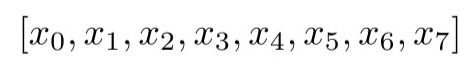
there’s a corresponding vector of the same length, which contains the individual values of the discrete Fourier transform of these numbers

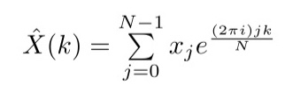
Which can be calculated via the DFT
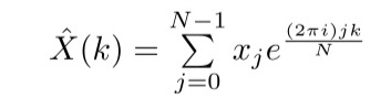
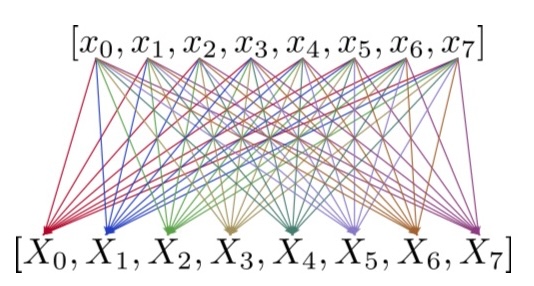
Where N is the length of the vector of numbers and k is a number between 0 and N-1. However, a naive implementation of the above is computationally very expensive; drawing out the contributions of the initial data points to the calculation of each Fourier transform value, we can see that this has complexity O(n²)
However, there’s a very clever alternative that has been the workhorse of digital Fourier transforms for decades. It’s called the Fast Fourier Transform.
The Fast Fourier Transform
The Fast Fourier Transform (FFT) works by breaking (or “decomposing”) a data-set down into many smaller individual sets, taking the discrete Fourier transforms of these smaller sets, and then progressively recombining them. This is a classical example of a “divide and conquer” algorithm, a mainstay of efficient computing. Here’s how this works.
Starting from the discrete Fourier transform, the FFT algorithm breaks the input data into two groups; those with even indices (x0, x2 etc) and those with odd indices. It calculates the DFT of those groups and then combines them to generate the full DFT. This core idea, that larger DFTs can be built out of smaller DFTs, can be repeated recursively.
The size of the smallest Fourier transform the algorithm performs is known as the radix of the decomposition. It’s typical for the FFT to decompose a data-set into radix-2, which means that the very smallest Fourier transforms are performed on pairs of values within each group, which are combined into progressively larger transforms.
At first glance, that doesn’t seem like it saves very much time; after all, we still need to perform multiple DFT operations! However, it becomes much clearer when we look at the flow of information and compare it to the O(n²)DFT above.
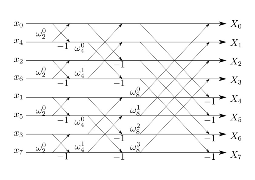
A “butterfly” diagram of the Fast Fourier transform that shows how information about smaller DFTs is progressively recombined to form a larger FT
So why does this approach work? Well, the FFT is dependent upon symmetry. In the above diagram, the omega values represent what are known as “twiddle factors”.
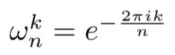
If you’re familiar with complex numbers and Euler’s identity, you’ll recognise this as simply being a complex number of magnitude 1 with a particular phase in complex space. We can recognise these twiddle factors from the DFT equation:
For an 8-point DFT, explicitly drawing out the twiddle factors for, say, the 8th input data point looks like this:
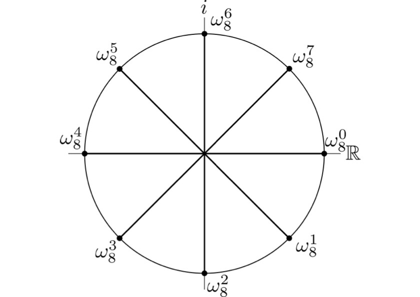
Drawn this way, we can clearly see that half of the factors are the symmetric opposite of the other half, varying by a phase of π. For a 4-point DFT, the diagram is much simpler;
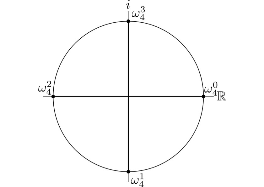
And for a 2-point DFT simpler still, while retaining the same kind of symmetry.
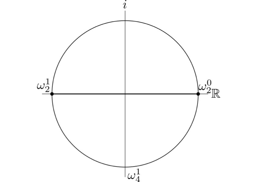
For a sequence of values of length N, the naive DFT requires the calculation of N output samples in the frequency domain. By making use of symmetry we only need to calculate half of the twiddle factors and we still gain all the information we need to calculate the next recursion!
So for our sequence of 8 values, only 24 operations need to be performed. For n inputs, this is O(n log n) operations, much fewer than the 64 operations required for the “naive” O(n²) DFT.
The difference between 24 and 64 operations might not seem like much, but when the amount of data increases, things quickly add up; for a 1024-element input, the FFT requires 10,240 operations compared to the 1,056,784 operations required by the DFT. At this scale, the FFT is 100 times faster, and continues to improve in relative performance as the inputs get larger.
This efficiency in calculating the Fourier transform makes the FFT arguably one of the most important algorithms in history. Without it, many essential tasks in computing, engineering and science would be much slower to compute.
However, we have an optical system in which any excess calculations are solved instantly through the properties of light. Aside from being incredibly quick, this also means that we don’t need to decompose to a radix any smaller than the maximum resolution of the system. We will however need to perform a similar process to reconstitute the bigger grid, so the use of an optical system will still have a similar structure to that of the Cooley-Tukey method. Despite this, the algorithmic complexity of the optical Fourier transform is still superior to the Cooley-Tukey method, even when working with a larger grid. We’ll show why that is below.
Computing a “large” discrete Fourier transform from a “small” one: extending the Cooley-Tukey FFT
To summarise the above, the Cooley-Tukey Fast Fourier Transform (FFT) is an algorithm used to compute a discrete Fourier transform with complexity O(N log N), where N is the number of entries. It is often used to compute one-dimensional Fourier transforms on electronic hardware where the fundamental operations are scalar additions and multiplications.
Here, we’re going to take the ideas behind the FFT, and show how we can apply them to calculating larger Fourier transforms using an optical system.
(This section is a bit heavier on mathematical details than the rest of the article. You can safely jump to the end where we give the main result if you are interested in the high-level idea rather than the explicit algorithm.)
Before that, we need to specify the problem and introduce some notation which will be helpful:
- We consider the two-dimensional discrete Fourier transform of a grid of discrete values where the number of values in each direction are set by some positive integers Nx and Ny. Two-dimensional arrays of real or complex numbers with the same shape will be denoted by bold capital Latin letters, and their coefficients with the non-bold version and two indices denoting their positions.
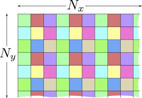
- We denote by FT the discrete two-dimensional Fourier transform. For an array A and each pair of integers (j,k) such that 1≤j≤Nx and 1≤k≤Ny, the 2-dimensional discrete Fourier transform is:

- We assume the device we work with has a rectangular input array of pixels, with sides given by two positive integers nx and ny. Two-dimensional arrays of real or complex numbers with the same shape will be denoted by bold lowercase letters.
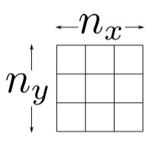
An example of a grid indicating device dimensions. Here, we’ll use a 3×3 grid to make things easier to demonstrate, although in practice the resolution of the optical system is larger.
- We denote by OFT the optical Fourier transform. For the sake of simplicity, we assume the OFT is an exact two-dimensional discrete Fourier transform defined in the same way as above. Let A be an array of shape (Nx,Ny). For each integer i between 1 and dx and j between 1 and dy, we define the sub-array aʲᵏ of shape (nx,ny) by:

- For an array a and pair of integers (j,k) such that 1≤j≤nx and 1≤k≤ny, the optical Fourier transform of a is:

- Finally, we assume that Nx is a multiple of nx and that Ny is a multiple of ny. We define the ratios dx = Nx / nx and dy = Ny / ny.
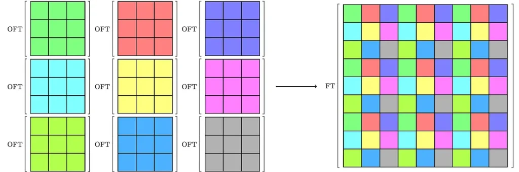
The question we are dealing with in this article is: Given a device which can perform a discrete optical Fourier transform, how can one reconstruct an arbitrary-sized FT function? Here, we present a solution in three steps: divide the input into dx dy smaller arrays of shape nx by ny, perform an OFT on each of them, and recombine the results. This is illustrated schematically in the figures below.
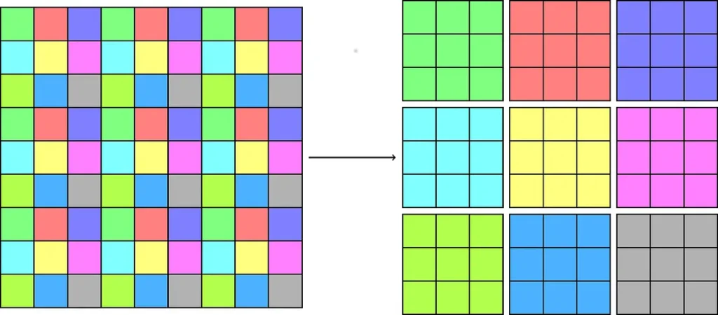
Illustration of the separation of a large array into smaller arrays, each of which corresponds to a different colour. The optical Fourier transform is applied to each small array, and the results are combined to yield the Fourier transform of the original one. Here, we’re showing how this would work for a device with a resolution of 3×3, to make things easier to see.
Animated sketch of the separation of a large array into smaller arrays.
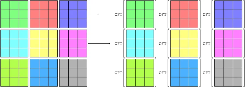
We then take the Fourier transform of each of the sub-arrays using the optical device.
Finally, the results are combined to yield the Fourier transform of the original array.
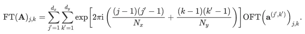
Let us assume we have computed the optical Fourier transform of each of these sub-arrays. Then, the Fourier transform of A can be computed as follows. Using the definition of the FT function and decomposing each integer between 1 and Nx (and respectively between 1 and Ny) in the right-hand side as multiple of dx and dy, plus the remainder of the Euclidean division by dx and dy, we have:

This may be rewritten using the smaller arrays we just defined as:

Using the property that exp(c1+c2) = exp(c1) exp(c2) for any two complex numbers c1 and c2, this becomes:

Performing the last two sums is equivalent to computing the optical Fourier transform of the array aʲ’ᵏ’. So,
In this equation, the array indices are assumed to be periodic (with period equal to the size of the array in the corresponding direction) in order to (slightly) simplify the notation. The indices i and j of the right-most array should be taken modulo and nx and ny, respectively.
This expression can be simplified in the following way. Let us define the two arrays with respective shapes Nx by dx and Ny by dy by:

and

Then,

We can now also estimate the complexity C of this calculation. Let us call C(OFT) the complexity of each OFT operation. There are nx ny such operations and then dx dy terms to sum for each coefficient. The complexity of the full calculation is thus O((Nx Ny + C(OFT)) dx dy). In general, C(OFT) will be much smaller than Nx Ny for large images. Asymptotically, the complexity thus becomes O(Nx Ny dx dy). This is better than the naive Fourier transform approach (which has complexity O(Nx² Ny²)) by a factor nx ny.
This result can be further improved by performing the decomposition iteratively several times. Indeed, there is nothing special about the use of the OFT function in the above calculation; just like the FFT, we’re performing a Fourier transform on a subset of the full array.
Let us assume, for definiteness, that there exists a positive integer m such that Nx = 2ᵐ nx and Ny = 2ᵐ ny. Then, the Fourier transform of A can be computed by first separating A into 4 sub-arrays (the number of recombination operations to reconstruct the full result from their Fourier transforms will be 4 Nx Ny), and then each sub-array in 4 smaller arrays (requiring again 4 Nx Ny recombination operations),… After m such subdivisions, we perform the 2²ᵐ optical Fourier transform on each sub-array of shape (nx,ny) and recombine the results. The total number of operations scales as O(4 m Nx Ny + 2²ᵐ C(OFT)). It may be rewritten using the total number N = Nx Ny of coefficients as

Since C(OFT) is at most linear in nx ny, this gives

In short, despite the fact that we need multiple frames to process a larger array, the time complexity of an optical Fourier transform is still less than the O(N log N) scaling of the Cooley-Tukey approach for large values of nx ny!