Optical computing for predicting vortex formation
We are developing a novel computing hardware solution that combines silicon photonics with free-space optics to perform a specific but highly useful mathematical operation (the Fourier transform) much faster than is possible on standard electronic hardware, while using far less energy.
Our technology has a vast range of uses in computing applications both new and old, and we test our hardware across as many of these applications as possible. This is partially to ensure that there are no limits to what the system can achieve when compared against conventional electronics, but at the same time this process also lays out a roadmap for the use of the technology in the applications of tomorrow.
In three of our previous articles, we showed how the hardware under development at Optalysys can be used to simulate physical systems more efficiently. We have also recently shown how the optical device can be used to perform Fourier transforms in arbitrary dimensions, thus allowing us to accelerate simulations using Fourier transforms in 1D, 2D, 3D, or even higher dimensions. We call our system the Echip demonstrator, because it is a prototype version of the actual Echip design.
Partial Differential Equations and Deep Learning
Aparticularly interesting application of deep learning is in the resolution of partial differential equations. As we have discussed before, this is hugely important in many fields of fundamental science and engineering. Sometimes, these equations can be solved exactly with pen, paper, and some algebraic gymnastics. In most cases, however, no solution can be found this way. The best way to proceed is then to solve the equations numerically.
Many problems involving partial differential equations can be solved using Fourier transform techniques where optical computing can already offer an advantage, and Optalysys has a history in this sector. However, it was recently proposed that a deep learning approach to solving partial differential equations could offer significant advantages over standard methods¹. In particular, deep networks can be trained to compute how the solution evolves over a potentially large time in a single evaluation, while standard algorithms require solving over time in many small intervals, a tactic that involves huge computational expense.
In our latest article on the subject, we illustrated how this idea works, taking as example the Navier-Stokes fluid dynamics equation in two dimensions and showing how a neural network can help to reconstruct the global dynamics of the flow.
In this article, we want to push this idea further and see whether deep neural networks can be used in combination with our existing hardware to detect the formation of small features, such as vortices, when the simulated domain is much larger. We will concentrate on the 2D case as an illustration and see how it can be used to build neural networks for detecting and predicting the formation of vortices, a task which is highly sensitive to the accuracy of a machine learning approach.
We begin by introducing a technique that will allow us to generate a dataset of many solutions. We then build a neural network that can detect the presence of these vortices in each solution, and finally one which can predict the formation of vortices at a later time even if there are none present in the initial conditions. We compare the performance of this network when run on conventional electronics and when using the Echip demonstrator to show that equivalent accuracy can be achieved.
The ability to predict where and when a vortex will form is a significant use-case for computational fluid dynamics which currently relies upon compute-and-energy intensive methods to solve the partial differential equations that govern fluid motion. By pairing a novel approach to PDE solving with highly efficient hardware, we provide a glimpse of a future in which a combination of AI and our new hardware drastically changes the scope and scale of physical simulations.
The Gross-Pitaevskii Equation
Use cases
The Gross-Pitaevskii equation (GPE) was named after Eugene P. Gross and Lev P. Pitaevskii for their work on the quantum behaviour of systems of particles called bosons.
The main application domain of the GPE is in fundamental physics, where it is used to model the quantum behaviour of atoms. Indeed, some species of atoms (specifically, atoms with an even number of neutrons) can, under certain conditions², form a peculiar state of matter called a Bose-Einstein condensate. This condensate can be described at the quantum level by a complex-valued function of time and space, sometimes called the ‘condensate wave function’, which is a solution of the GPE. You can think of this function as an equivalent to the usual wave functions in quantum mechanics, which are solutions of the Schrödinger equation. The main difference is that, while these wave functions each relate to a single particle, the ‘condensate wave function’ describes a set of possibly many particles. In short, the GPE can thus be used to perform quantum simulations that involve many particles.
This equation can also model other physical phenomena, such as deep water waves, pulse propagation in an optical fibre, and modulation instabilities. In this article, we use the GPE to generate a data-set that contains flow-field vortices.
Mathematical definition
The Gross-Pitaevskii equation describing the behaviour of low-density cold atoms with short-range interactions may be written as:

Let us take a moment to explain the symbols used in this equation:
- i is a complex number whose square is -1.
- ħ is a positive constant, called the reduced Planck constant.
- m (also a positive number) is the mass of each atom.
- g is a real number (which can be positive, negative, or formally 0) which determines the strength of interactions between atoms. The atoms tend to repel each others if g >0 or attract each others if g < 0 (or do not interact at all if g = 0).
- ψ is a complex field; put informally, a complex number whose value depends both on the position in space and time where it is defined. Mathematically, it is a function from ℝ × ℝ³ to ℂ, where the first ‘ℝ’ (the set of real numbers) encodes time, ℝ³ (whose elements are made of three real numbers) encodes the position in space, and ℂ is the set of complex numbers.
- V is a real field, i.e., a function from ℝ × ℝ³ (or just ℝ³ if it does not depend on time) to ℝ. It represents the external potential, i.e., the potential energy that an atom would have in the absence of other atoms.
- ∂ₜ denotes the derivative with respect to time.
- Δ is the Laplacian operator, i.e. the sum of the second derivatives in the space directions.
(The same equation can be used in the other contexts mentioned above, with different interpretations for the constants ħ, m, and g and the function V.)
In the cold atoms context, ψ is not itself an observable quantity: you cannot see it nor otherwise measure directly. However, it is closely related to two important physical quantities:
- the atom density, proportional to the number of atoms per unit volume, is given by its squared modulus,
- the local velocity of atoms is proportional to the gradient of its phase.
In the following, to reduce the number of parameters, we work in a unit system where the constants ħ, m, and g are equal to 1. (This is always possible provided g is positive, i.e., that the interactions between atoms are repulsive.) The same procedure would work in other unit systems, for arbitrary values of these parameters.
Neural Networks and Vortices
What is a vortex?
Formally, in the context of the 2D GPE, a vortex may be defined as a point where the density vanishes and around which the phase changes by 2π (or a non-zero multiple of it).³ The second point is illustrated in the figure below:
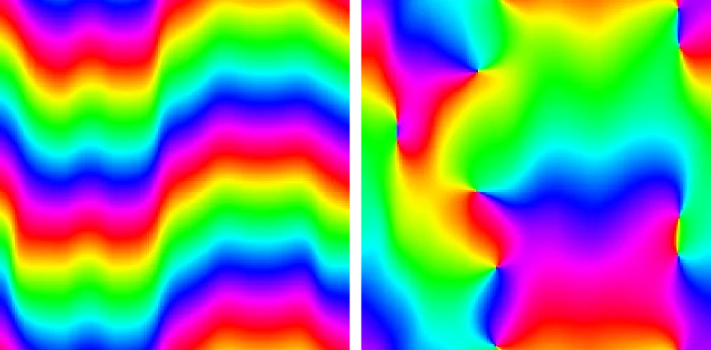
Two examples of snapshots of the phase of a complex field in 2 space dimensions. The left one has no vortex, while the right one has 10 vortices.
Another (equivalent) way to see a vortex is as a flux of atoms orbiting around a central point; in the figure below, we show the direction of the atoms velocity as small black arrows:
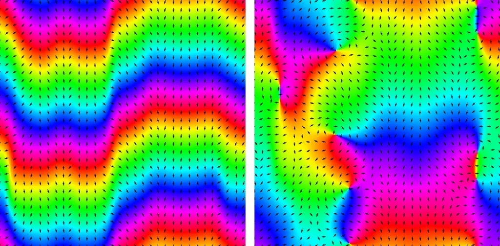
The two above images with the direction of the velocity (black arrows).
The velocity is proportional to the gradient of the phase. Around a vortex, it will thus be (approximately) circular.
Simulations
We generated training data by solving the GPE 20,000 times with different initial conditions. The equation was discretized in space and time and, at each time step, the differential operators were evaluated on the Fourier transform of the field (the resolution method was very close to the techniques described in these articles, where more details can be found).
For definiteness, we set the parameters ħ, m, and g to 1. The numerical grid had a size 250 by 250, with a spatial step of 0.076. The field was evolved for 2,400 time steps with size 0.01. The potential was a simple step-like function, equal to -1 for y < 0 and for +1 for y > 0, where y is one of the space coordinates, which can model a cliff-like obstacle.
The initial conditions were chosen as follows. Two numbers A and σ were chosen randomly (independently for each simulation) in the intervals [-0.2,0.2] and [0.5,2.5], as well as two integers nx and ny between -3 and 3. At time t = 0, the density, usually denoted by the Greek letter ρ, was equal to

and the velocity, often noted v, was

These constraints were chosen so that vortices appear in about 70% of the simulations. The mean number of vortices (including simulations where none appears) is between 6 and 7. 90% of the simulations were used for training, and the remaining 10% were used for testing.
Vortices were counted automatically by looking at the phase differences between nearby pixels. Let h be the height of the image and w its width. For each integer i between 1 and h-1 and each integer j between 1 and w-1, we consider that there is a vortex inside the square delimited by the positions (i,j), (i+1,j), (i+1,j+1), and (i,j+1) if the phase differences between positions (i,j) and (i,j+1), (i,j+1) and (i+1,j+1), (i+1,j+1) and (i+1,j), and (i+1,j) and (i,j) have the same sign.
Training on a large number of images
The GPU used to train the networks (an NVIDIA GeForce RTX 2070 SUPER) has only 8GB of memory, which is not quite enough to store all the training images. To get around this difficulty, we selected a subset of 2,000 training images at the start of each epoch and updated the network weights using these images only. The choice was made at random for each epoch, so that each training image was used about once every 9 epochs.
Training a neural network to count vortices
The first problem we consider is vortex detection: given an image of a field configuration such as those shown above, the network should count and output the number of vortices. We use a standard convolutional neural network, with ReLU activation function for each layer except the last layer. We tried different sets of hyperparameters and found that a very small network with only one convolution layer and one hidden dense layer seems to give good results. The hyperparameters are summarised in the following table:
| Layer type | Kernels / Neurons | Activation |
|---|---|---|
| Convolution | 4x3x3 | ReLU |
| Dense | 10 | ReLU |
| Dense | 1 | None |
The following plot shows results obtained when training the network on a GPU. We use the mean squared error as the loss function, i.e., the squared difference between the number of vortices counted by the network and the “true” number as determined by the labelling process.
The next plot shows the results obtained when using the Optalysys Echip demonstrator to perform the convolutions:
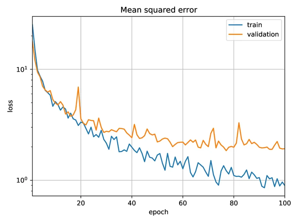
Mean squared error as a function of the number of epochs for a convolutional neural network trained to count vortices in a snapshot of a simulation. The training and inference are done using data from the Echip demonstrator.
The next plot shows the results obtained when using the Optalysys Echip demonstrator to perform the convolutions:
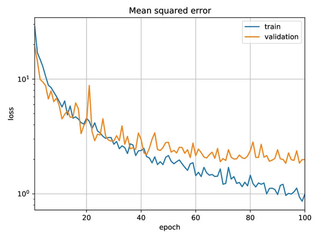
Mean squared error as a function of the number of epochs for a convolutional neural network trained to count vortices in a snapshot of a simulation. The training and inference are done using data from the Echip demonstrator.
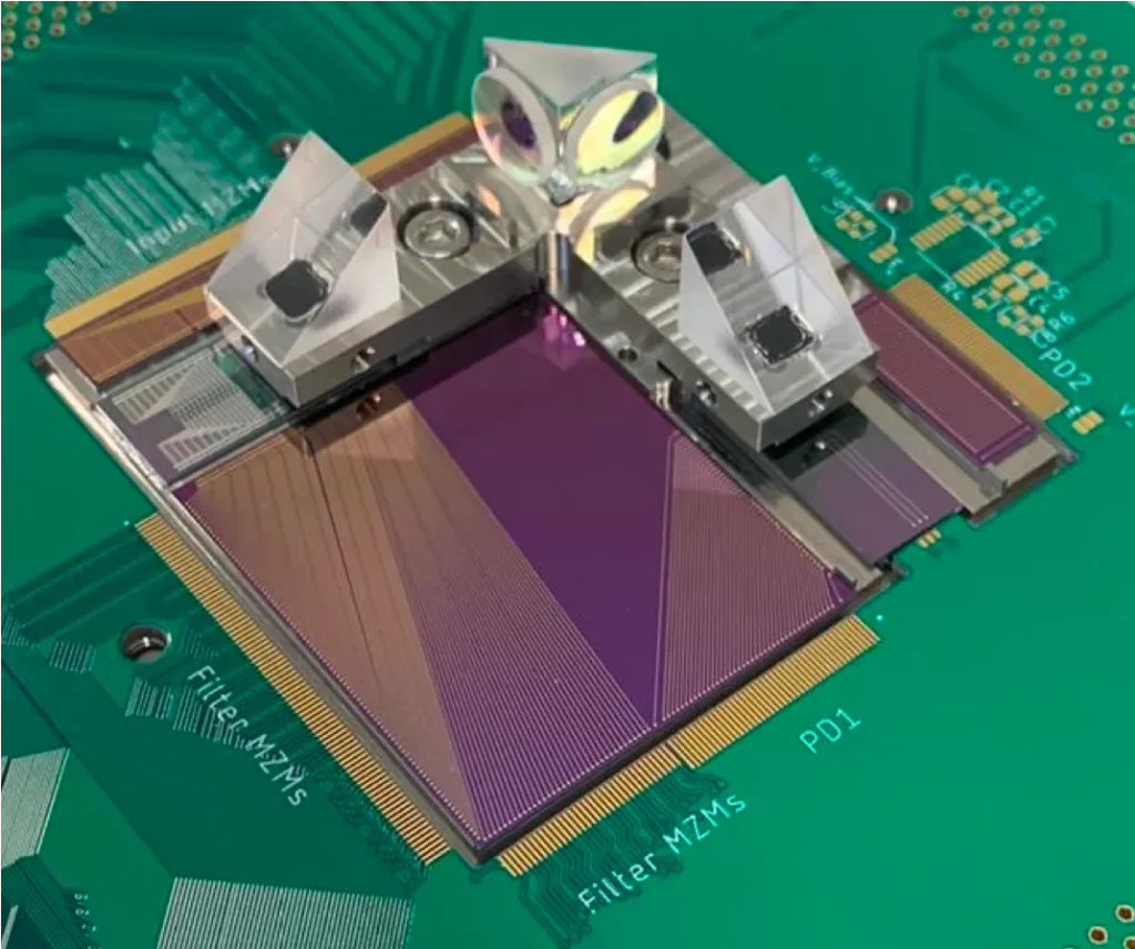
The Echip demonstrator currently in use at Optalysys.
In both cases, the (validation) mean squared error after 100 epochs is close to 2, corresponding to an error in the vortex count slightly above 1. This is close to the error of the function used to label the simulations, due to the difficulty in detecting vortices close to each other, and notably smaller than the averaged number of vortices in a simulation (which is a bit above 6.3).
If the data were correctly labelled, it is likely that the accuracy could be improved by modifying the network to reduce the overfitting. However, the function used to label them can easily miss vortices when the phase varies too fast. The labelling of data is thus expected to be off by about one or two on images with many vortices. For this reason, there is little point in reaching a better accuracy on this data.
Training a Neural Network to Predict Whether Vortices Will Form
We now turn to the more difficult problem of predicting the formation of vortices from initial conditions where none have (yet) appeared. The task the neural network should solve is the following: given a picture of the density and phase of the field at one time t1, it must determine whether there will be vortices at a later time t2. We concentrate on the case where there is no vortex at time t1. Otherwise, the problem would be too easy: since vortices rarely disappear (in our set-up, the only way a vortex can disappear is by colliding with another), the presence of vortices at time t1 would be a very strong indication that they are still present at time t2. With the condition that no vortex is present at time t1, the network needs to learn the features that lead to vortex formation, and should not simply detect whether vortices are already present.
We again use convolutional neural networks, with a few convolutional layers followed by dense layers. All layers have a ReLU activation function, except the last dense layer, with only one neuron. We used three different architectures. The first one is a ‘small’ network with two convolutional layers and a single hidden dense layer. The structure is given in the table below:
| Layer type | Kernels / Neurons | Activation |
|---|---|---|
| Convolution | 4×3×3 | ReLU |
| Convolution | 4×3×3 | ReLU |
| Dense | 10 | ReLU |
| Dense | 1 | None |
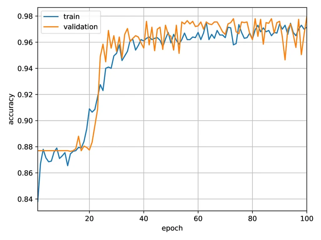
The figure below shows the evolution of the accuracy during training:
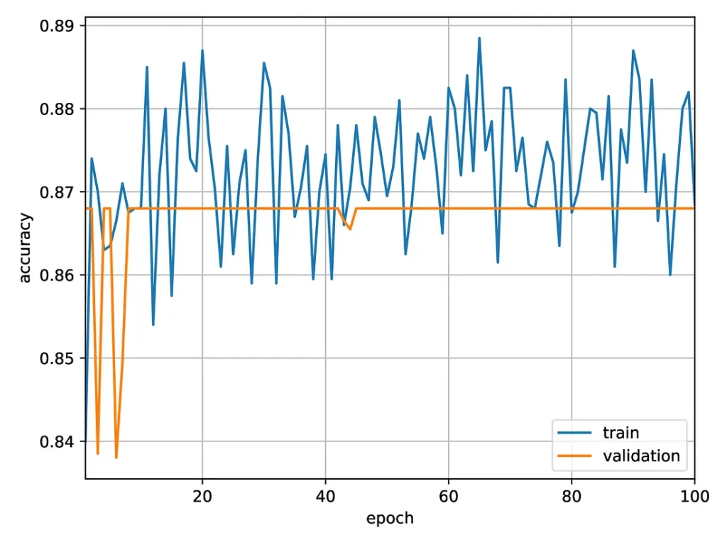
Accuracy of a ‘small’ neural network for predicting the formation of vortices.
The network seems to be stuck on a plateau, with a validation accuracy just below 87%. The network is learning something: since vortices appear in about 70% of the simulations we use for both training and validation, achieving an accuracy above 80% requires it to detect features that are somewhat predictive of vortex formation. However, there is definitely room for improvement.
We then re-did the same experiment using a larger network with updated hyperparameters as given below:
| Layer type | Kernels / Neurons | Activation |
|---|---|---|
| Convolution | 32×3×3 | ReLU |
| Convolution | 64×3×3 | ReLU |
| Convolution | 128×3×3 | ReLU |
| Dense | 100 | ReLU |
| Dense | 20 | ReLU |
| Dense | 1 | None |
This network yields significantly better results:
Accuracy of a ‘large’ neural network for predicting the formation of vortices.
At later times, the accuracy oscillates between 95% and 98%. It would likely be possible to improve the accuracy by fine-tuning the parameters or adding a learning rate optimizer. However, here we are mostly interested in comparing the electronic results with those obtained using the Optalysys Echip demonstrator. We thus consider that an accuracy above 95% is sufficient, and would like to see if the same network can give similar performances when run optically.
To make a fair comparison, we need to check that we have not added too many parameters. The number of parameters in the ‘large’ network is nearly two orders of magnitude higher than that of the ‘small’ one. To get a feel for whether this is too much, we did a third experiment with a ‘medium’ network with the following hyperparameters:
| Layer type | Kernels / Neurons | Activation |
|---|---|---|
| Convolution | 4×3×3 | ReLU |
| Convolution | 8×3×3 | ReLU |
| Convolution | 16×3×3 | ReLU |
| Dense | 100 | ReLU |
| Dense | 20 | ReLU |
| Dense | 1 | None |
The number of parameters is close to the geometric mean of the previous two (see table below). When trained electronically, it yields an accuracy of about 97%, close to that of previous network. Increasing the number of parameters thus does not seem to improve the results.
We trained and evaluated this ‘medium’ network using the Echip demonstrator, with the following results:

After 150 epochs, the network reaches an accuracy of 97%, equivalent to that of the electronic version.
Results for the four different networks are summarised in the table below, with the error bars estimated from the amplitude of the fluctuations in the last few epochs:
| Model | Number of parameters | Accuracy after 100 epochs |
|---|---|---|
| small CNN (electronic) | 154005 | (86.5±1)% |
| medium CNN (electronic) | 1541281 | (97±1)% |
| large CNN (electronic) | 12395901 | (97±1)% |
| medium CNN (optical) | 1541281 | (97±1)% |
Outlook
In this article, we have seen how a neural network can be trained to detect vortices in a snapshot of a GPE simulation or to predict the formation of vortices from a situation where they have not (or not yet) appeared. We trained several versions of the networks, both electronically and using the Optalysys Echip demonstrator for the convolutions. Both the electronic and optical versions reached an accuracy above 95%. One can draw two main conclusions from these results:
- First, convolutional neural networks can be used to efficiently detect and predict the formation of small-scale feature such as vortices in simulations of partial differential equations with a good accuracy.
- Second, networks using the optical Fourier transform to perform the convolution perform as well as their fully electronic counterparts.
The second point is particularly important as use of the optical Fourier transform can make these networks significantly faster and more energy efficient. In practice, large simulations are usually limited by the time needed to run them or by the energy consumption (which are often two sides of the same coin: you can increase the speed at the cost of a higher power usage by adding more compute cores until the limit of Amdahl’s law is reached). Using the optical Fourier transform would thus allow larger networks to simulate more complex systems with better resolution or over longer time-scales than could be achieved solely with electronic means.
We plan to extend this work in two directions. First, we can study similar problems in more realistic models, for instance in three dimensions or using the Navier-Stokes equations. Second, we will implement similar neural networks on the next-generation Optalysys Echip demonstrator. The latter will be able to do large Fourier transforms faster than the current version, which will help in dealing with larger and more realistic models in real-world applications.
¹ See https://arxiv.org/pdf/1910.03193.pdf and https://arxiv.org/pdf/2010.08895.pdf
² Specifically, there are three conditions: the atoms must be sufficiently cold for thermal effects to be small, have no long-range interactions, and be sufficiently dilute.
³ More information on vortices can be found in these slides by Sandro Stringari, one of the main contributors to the theory of Bose-Einstein condensation: https://www.mcqm.cond-math.it/ewExternalFiles/stringari.pdf