
Transformer networks are an incredibly powerful deep learning architecture and they can be truly enormous. GPT-3, the natural language model that made headlines last year both for its exceptional performance and vast number of parameters, is a transformer network. However, training these networks takes up vast amounts of computing time, which in turn consumes a significant amount of power. As of 2019, GPU-powered training of a single large transformer network with neural architecture search could produce upwards of 625,155 lbs of CO2. This is equivalent to the CO2 released by 5 or so cars over the course of their lifetime.
GPT-3 is considerably larger than any of the models made before 2019, and Google have recently unveiled their own NLP network which is 9 times larger than GPT-3. Standard electronic hardware may be still be becoming more efficient and powerful, but not at a rate that can offset the explosive growth in AI processing requirements. Cutting down on the power consumed by AI is therefore critical for hitting global emissions targets.
In this article, we show that the transformer networks can be trained and evaluated using convolutional methods. This technique allows us to implement transformer networks and related lambda networks on our ultra-efficient Fourier-optical computing architecture, opening the door to an order of magnitude improvement in power consumption for these tools with no loss in performance.
Article breakdown:
We begin by describing previous attempts at extracting information from long sequences of data and how transformers solved some of the problems with these approaches.
We describe how the underlying attention-based method works in a transformer, and then explain how this method can be expressed in convolutional terms.
We then show how we implemented these techniques on our optical processing device for both transformer and lambda layer networks, and demonstrate that Fourier-optical processing techniques are an ultra-efficient way of performing the calculations that drive these methods.
Transformer networks, also called transformers, are deep learning models first proposed in 2017 by researchers from Google Brain, Google Research, and the University of Toronto to deal with long sequences of data. The previous state-of-the-art in Machine Learning for sequential data mostly consisted of Recurrent Neural Networks (RNNs) with Long-Short Term Memory cells or Gated Recurrent Units, or Convolutional Neural Networks (CNNs), which had shown promising results in some applications like translation of short texts but suffered from several issues.
The first one was parallelization: since most RNNs need to deal with the input data sequentially, they don’t benefit much from the parallelization capabilities of GPUs or TPUs which have been crucial in accelerating other types of neural networks.
The second issue was the vanishing gradient problem: CNNs (and, to a lesser extent, some RNNs) are very good at detecting local patterns in sequences or images but require many layers (or passes) to detect correlations between two words or pixels which are far apart. Since the gradient of the loss function tends to decrease from one layer to the next, this makes it hard to learn such correlations.
Transformer networks make use of a different mechanism, called attention, which can be efficiently parallelized and deals with correlations between distant inputs in a single layer (at least in principle; in practice, the number of correlations which can be encoded in a single layer is limited by the memory requirement, which is quadratic in the number of inputs¹). The attention mechanism was actually first used in RNNs to help them learn long-distance correlations, but it was then shown that, paraphrasing the title of the paper where transformers were first proposed, the attention mechanism is (nearly) all you need.
The first and foremost domain of application of transformer networks is natural language processing, comprising (among other tasks) text translation, analysis, and generation. Among the best-known models are the Bidirectional Encoder Representations from Transformers (BERT), developed by Google and used (among other application and lines of academic research) to process Google searches (it was first limited to English searches, but was then extended to other languages), and the Generative Pre-Trained Transformer 3 (GPT-3) developed by OpenAI for text generation.
However transformers are increasingly used for tasks outside what is usually seen as the boundary of natural language processing, such as image classification (although CNNs are still dominant for problems combining locality with translation invariance, as in image detection and classification problems) or image generation from captions, as exemplified by the DALL·E² version of GPT-3.
The main ingredient of a transformer network is the attention mechanism. Given a long series of inputs, it is a means of determining how much weight should be given to each element in the context of the sequence.
One of the most common forms of attention is self-attention, which we now briefly describe. (A more detailed description with examples can be found in this Medium article from towards data science.) Self-attention consists of one or more attention heads. Each attention head is a triplet of matrices (Q,K,V) with the same size, called the query, key, and value weights. Each input i is converted into a vector xᵢ, called word embedding, from which we define query qᵢ, key kᵢ, and value vᵢ vectors by the formulae: qᵢ = Q xᵢ, kᵢ = K xᵢ, and vᵢ = V xᵢ. The attention wᵢⱼ between inputs i and j is the scalar product of the query qᵢ associated with the first one and the key kⱼ associated with the second one. The output of the attention head for the input i is then

i.e., the average of the value vectors with weights given by the exponential of the attention divided by the square root of the size k of each vector. (Dividing the attention by this square root seems to make the training more stable. The reason is that, in general, the magnitude of the attention is of the same order as this square root, so that dividing by the latter gives numbers of order 1.)
As an illustration, we show here a simple Python implementation for a standard self-attention class, written in PyTorch. The parameters k and hrepresent the length of each word embedding and number of attention heads, respectively. The code shown below draws inspiration from the attention layer in Peter Bloem’s GitHub repository.
import torch
from torch import nn
import torch.nn.functional as F

class SelfAttention(nn.Module):

    def __init__(self, k, h):

        super().__init__()

        # set the parameters k and h
        self.k, self.h = k, h

        # functions to compute the queries, keys, and values for all heads
        # Vectors obtained with all heads are concatenated into a single
        # vector.
        # Each function takes a vector of size k and returns a vector of size
        # k*h.
        self.toqueries = nn.Linear(k, k*h, bias=False)
        self.tokeys = nn.Linear(k, k*h, bias=False)
        self.tovalues = nn.Linear(k, k*h, bias=False)

        # function to turn each of the resulting vectors into a vector of size k
        # We allow a bias to be learned.
        self.unifyheads = nn.Linear(k*h, k)

    # forward pass
    def forward(self, x):

        # size of a mini-batch, number of vectors, and size of each vector
        b, t, k = x.size()

        # number of heads
        h = self.h

        # compute the queries, keys, and values, and separate each vector of
        # size h*k into h vectors of size k
        queries = self.toqueries(x).view(b, t, h, k)
        keys = self.tokeys(x).view(b, t, h, k)
        values = self.tovalues(x).view(b, t, h, k)

        # merge the head and batch dimensions
        queries = queries.transpose(1,2).reshape(b*h, t, k)
        keys = keys.transpose(1,2).reshape(b*h, t, k)
        values = values.transpose(1,2).reshape(b*h, t, k)

        # scale the queries and keys
        # (applying the scaling now rather than later saves memory for long
        # sequences)
        queries /= k ** (1/4)
        keys /= k ** (1/4)

        # dot product of the queries and keys
        dot = torch.bmm(queries, keys.transpose(1,2))

        # apply the softmax function
        dot = F.softmax(dot, dim=2)

        # apply the self-attention to the values
        out = torch.bmm(dot, values).view(b, h, t, k)

        # move the h index back to position 2 and aggregate it with k
        out = out.transpose(1,2).reshape(b, t, h*k)

        # unify the heads
        return self.unifyheads(out)

The full transformer network we used in this study consists of 6 blocks and one final linear layer generating the predictions, plus an input layer with position embedding. (These layers are identical for the five versions of the network whose results are reported below.) Each block is constructed as an attention layer followed by a perceptron with ReLU activation function and a normalisation layer. The PyTorch code for the full network is given in an appendix at the end of this article.
As we explained in our previous articles, Optalysys’ optical chips will revolutionise optical computing by providing a much more time- and energy-efficient way to perform Fourier transforms and convolutions than is possible on electronic hardware because of the O(1) scaling of the optical Fourier transform and the energy savings from performing calculations in light. We have previously explained how it can be used in lattice-based cryptography and Bayesian neural networks. This is particularly useful for CNNs, which, as their name indicates, heavily rely on convolution operations. But could optical convolutions also be used for other machine-learning models?
Given the recent rise of transformer networks for a wide variety of tasks, notably in natural language processing, the ability to perform part of the training and/or inference optically would significantly expand the range of applications of optical computing. There could also be inherent advantages to using the convolution operation, such as preservation of input structure and spatial/contextual relationships between inputs and outputs of network layers. In this section, we show that this is indeed possible. More precisely, the matrix-vector multiplications used to compute the query, key, and value vectors can be replaced by convolutions, which can be performed optically at reduced runtimes and energy consumption.
In the above code example, the nn.Linear functions are matrix-vector multiplications (plus a bias for the last one), with the matrix containing the weights to be learned. Let us now show the code for a similar layer with matrix-vector multiplications replaced by convolutions:
import torch
from torch import nn
import torch.nn.functional as F

class SelfAttention_Conv(nn.Module):

    def __init__(self, k, h):

        super().__init__()

        # set the parameters k and h
        self.k, self.h = k, h

        # functions to compute the queries, keys, and values for all heads
        # Vectors obtained with all heads are concatenated into a single
        # vector.
        self.toqueries = nn.Conv1d(1, h, k, bias=False)
        self.tokeys = nn.Conv1d(1, h, k, bias=False)
        self.tovalues = nn.Conv1d(1, h, k, bias=False)

    # forward pass
    def forward(self, x):

        # size of a mini-batch, number of vectors, and size of each vector
        b, t, k = x.size()

        # number of heads
        h = self.h

        # compute the queries, keys, and values, and separate each vector of
        # size h*k into h vectors of size k
        # x is concatenated with itself (with the last dimension reduced by 1)
        # to simulate periodic boundary conditions. (In an optical implementation,
        # this step will not need to be performed explicitly.)
        queries = self.toqueries(torch.cat([x,x[...,:-1]],-1)
                                      .view(b*t,1,2*k-1)).view(b, t, h, k)
        keys = self.tokeys(torch.cat([x,x[...,:-1]],-1)
                                .view(b*t,1,2*k-1)).view(b, t, h, k)
        values = self.tovalues(torch.cat([x,x[...,:-1]],-1)
                                    .view(b*t,1,2*k-1)).view(b, t, h, k)

        # merge the head and batch dimensions
        queries = queries.transpose(1,2).reshape(b*h, t, k)
        keys = keys.transpose(1,2).reshape(b*h, t, k)
        values = values.transpose(1,2).reshape(b*h, t, k)

        # scale the queries and keys
        # (applying the scaling now rather than later saves memory for long
        # sequences)
        queries /= k ** (1/4)
        keys /= k ** (1/4)

        # dot product of the queries and keys
        dot = torch.bmm(queries, keys.transpose(1,2))

        # apply the softmax function
        dot = F.softmax(dot, dim=2)

        # apply the self-attention to the values
        out = torch.bmm(dot, values).view(b, h, t, k)

        # unify the heads
        return torch.sum(out, dim=1)
The main difference is the replacement of the nn.Linear object by nn.Conv1d, which is a one-dimensional convolution, or by a simple sum in the last step of the forward pass.³ The modifications in the forward function are just here to ensure periodic boundary conditions are used for the convolution, as will be the case when performed using the optical device. This function thus simulates a layer that could use the optical convolution. However, to fully harvest the power of optical computing, it is best to work with two-dimensional convolutions. Fortunately, this requires only small changes to the code.
When working with two-dimensional convolutions, lines 35, 37, and 39 need to be modified so that periodic boundary conditions are imposed in the two directions. We also replace the parameter k by two numbers k₁ and k₂ representing the filter size in the two directions; the size k of the word embedding is then k = k₁ k₂. Apart from that, and the replacement of Conv1d by Conv2d, the code is identical:
import torch
from torch import nn
import torch.nn.functional as F

class SelfAttention_Conv2D(nn.Module):

    def __init__(self, k1, k2, h):

        super().__init__()

        # set the parameters k1, k2, and h
        # k1 and k2 give the size of the convolution kernels
        self.k1, self.k2, self.h = k1, k2, h

        # functions to compute the queries, keys, and values for all heads
        # Vectors obtained with all heads are concatenated into a single
        # vector.
        self.toqueries = nn.Conv2d(1, h, (k1,k2), bias=False)
        self.tokeys = nn.Conv2d(1, h, (k1,k2), bias=False)
        self.tovalues = nn.Conv2d(1, h, (k1,k2), bias=False)

    # forward pass
    def forward(self, x):

        # size of a mini-batch, number of vectors, and size of each vector
        b, t, k = x.size()
        k1, k2 = self.k1, self.k2

        # number of heads
        h = self.h

        # compute the queries, keys, and values, and separate each vector of
        # size h*k into h vectors of size k
        # concatenate x with itself in each direction (with the last
        # dimension reduced by 1) to simulate periodic boundary conditions
        queries = self.toqueries(x.view(b*t,1,k1,k2)
                                  .repeat(1,1,2,2)[:,:,:-1,:-1]).view(b,t,h,k1*k2)
        keys = self.tokeys(x.view(b*t,1,k1,k2)
                            .repeat(1,1,2,2)[:,:,:-1,:-1]).view(b,t,h,k1*k2)
        values = self.tovalues(x.view(b*t,1,k1,k2)
                                .repeat(1,1,2,2)[:,:,:-1,:-1]).view(b,t,h,k1*k2)

        # merge the head and batch dimensions
        queries = queries.transpose(1,2).reshape(b*h, t, k1*k2)
        keys = keys.transpose(1,2).reshape(b*h, t, k1*k2)
        values = values.transpose(1,2).reshape(b*h, t, k1*k2)

        # scale the queries and keys
        # (applying the scaling now rather than later saves memory for long
        # sequences)
        queries /= (k1*k2) ** (1/4)
        keys /= (k1*k2) ** (1/4)

        # dot product of the queries and keys
        dot = torch.bmm(queries, keys.transpose(1,2))

        # apply the softmax function
        dot = F.softmax(dot, dim=2)

        # apply the self-attention to the values
        out = torch.bmm(dot, values).view(b, h, t, k1*k2)

        # unify the heads
        return torch.sum(out, dim=1)
Of course, just being able to build transformer networks using convolutions does not necessarily mean that they will be useful. As we mentioned above, convolutions can in principle be performed optically with much smaller runtimes and energy consumption than electronic hardware requires for the same operations, or for matrix-vector multiplication. But running a network efficiently is only useful if said network can learn something! We thus need to show that the convolution-based transformer is useful for the kind of problems standard transformers are used for.
To this end, we repeated the experiment described in Peter Bloem’s GitHub repository and his blog post. It consists of a sentiment analysis task, where the aim is to determine whether a film review (without explicit rating) is positive or negative. Essentially, the network should “read” each review and output a number equal to 0 if it thinks the review is negative or 1 if it thinks it is positive. We used the IMDb dataset from the torchtext.datasetsmodule. For all the results reported below, the networks had 6 attention blocks with 8 attention heads each, an embedding size of 128 (except the third one, which has an embedding size of 121), and were trained on 20 epochs on an NVIDIA GeForce RTX 2070 SUPER GPU.
To check that the idea of using convolutions in transformer networks makes sense, we first trained a standard transformer and a transformer using one-dimensional convolutions on the same dataset and with the same word embedding size of 128. The figure below shows the validation accuracy for both networks:
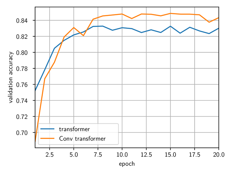
Comparison of the validation accuracy for a standard transformer network (blue line) and one using convolutions instead of matrix-vector multiplications (orange line).
Interestingly, the second network performs slightly better than the first one, reaching 84% accuracy versus 83% for the standard transformer. One should probably not pay too much attention to the difference, which might be erased by fine-tuning the parameters of the first network. (We did make sure that the parameters are close to the optimal choice, though, so it is unlikely that the standard transformer could perform much better.) However, it is a strong indication that a network using convolutions can perform at least as well as a standard transformer.
With a view to implementing the network on an optical processor, we have also tested it with two-dimensional convolution kernels. The figure below shows results obtained with a kernel size of 16 x 8 (chosen to give the same embedding size of 128).
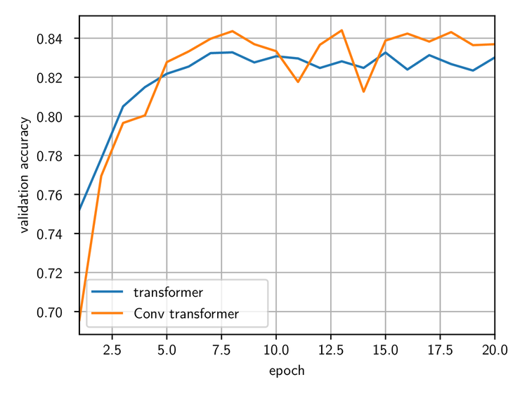
Comparison of the validation accuracy for a standard transformer network (blue line) and one using two-dimensional convolutions instead of matrix-vector multiplications (orange line).
The validation accuracy reached after 20 epochs is very close to that obtained with one-dimensional kernels. (The difference does not seem to be statistically significant.)
Finally, we did the same experiment with filter size 11×11, which is the size we expect to reach with our next optical chip. The figure below compares the validation accuracies obtained with the two different kernel sizes:
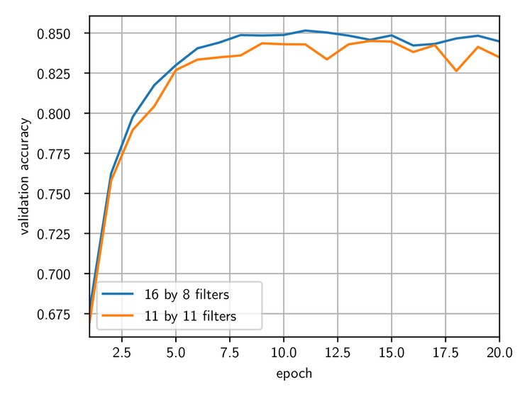
Comparison of the validation accuracy for transformer networks using 2-dimensional convolutions with different filter sizes.
The results are very close to those obtained with the previous kernel size, and still slightly better than those obtained with the standard transformer.
As we mentioned above, an important advantage of convolutions over matrix-vector multiplications is the possibility to perform them very efficiently using the optical Fourier transform, which reduces the complexity of the convolution to O(N), where N is the size of the input, and the runtime to O(1) using parallelization. But does a network trained using optics actually work in practice? We put this to the test. The following results were produced on our current Fourier engine demonstrator system as pictured below, and described in several of our previous articles.
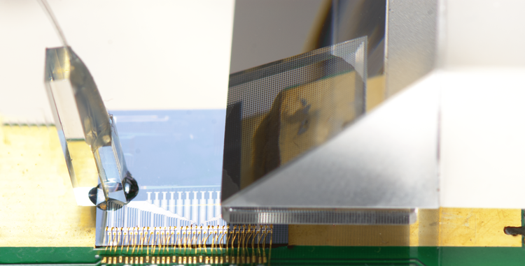
The current 5×5 Fourier Engine demonstrator. Light from a laser source (left of the figure) is split into several beams, passes through a silicon photonic chip where the desired input is encoded, and is sent to a lens performing the Fourier transform (right of the figure).
To make the setup as simple as possible and keep it close to the experiments we did with convolutional neural networks, we did not use periodic boundary conditions, so the kernel size was effectively 3 by 3. The evolution of the train and validation accuracies are shown in the plot below:
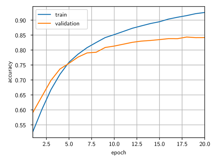
Train and validation accuracy for the convolution transformer trained using Optalysys’ optical device.
The network requires more epochs to reach a good accuracy; this seems to be due to the use of smaller kernels (we observed a similar slow-down when training a network electronically with kernels of the same size). More importantly, the accuracy reached after 20 epochs is a bit higher than 84%, which is as good as the best result we obtained electronically. This shows that transformer networks based on the optical Fourier transform can perform at least as well as their electronic counterpart — but at greatly increased speeds and smaller power usage!
These results, and others that will be presented in due course, make us confident that the optical device under development at Optalysys is a perfect fit for building transformer networks. We have explored here the possibility to use optical convolutions for computing the query, key, and value associated with each token in a self-attention layer, and showed that the network achieves results which are identical to or better than those obtained with standard transformers using matrix-vector multiplications. While an optical implementation could make transformers significantly more efficient (we estimate that convolutions currently take about 40% of the training time on a GPU), it is still a fairly conservative step: the resulting network has the same architecture as a standard transformer apart from the use of convolutions. We now turn to more ambitious ideas, with a view to replacing the dot product operations in the attention layers by a more time-, energy-, and memory-efficient variant using the unique features of our optical device.
The literature suggests that if convolutions are mixed with attention-like mechanisms, then state of the art image classification results may be achieved. The paper ‘Lambda Networks — Modelling Long-range Interactions Without Attention’ introduced the Lambda layer which has achieved great results on the ImageNet dataset. The primary obstacle that hinders the use of vanilla transformer networks for image classification is the undesirable quadratic scaling of the architecture. Such scaling is undesirable for runtime, but more importantly for memory. Quadratic memory scaling renders operations on large batches of data impossible, meaning that parallel hardware architectures cannot be exploited (like how GPUs can accelerate CNNs). This has been a huge stumbling block for the application of highly promising transformer architectures to high resolution images.
Lambda layers are able to attain long-range (global) interactions without incurring the quadratic scaling penalty. As mentioned previously, in a normal transformer, the Query and Key matrices are multiplied together leading to quadratic (with respect to sequence length) algorithmic complexity. Lambda layers do things differently. The core idea is that global contexts and positional embedding can be transformed into linear functions or Lambdas before they interact with the queries. See the below equations for a more detailed explanation.
In a normal transformer architecture, queries Q and keys K are obtained by transforming the input sequence X via weight matrices:

Attention is calculated by multiplying Q and K and softmaxing:

This operation scales quadratically in memory and compute, and must be recomputed for each item in the batch.
In a lambda layer, queries are generated in the same way:

These operations allow for a global, content based encoding which is similar to attention, but that does not scale quadratically. A positional encoding lambda P is also created, this combines the values (V) with an embedding matrix that is optimised during training:

The embedding matrix E describes relations between each element of a sequence and each other element. The content lambda is then summed with the positional lambda P that captures relevant positional information in the input sequence, giving the output Y:

In this way the scaling of the content-based interactions in Lambda layers is linear with respect to sequence length, stepping away from quadratic runtime scaling by compressing the input using trainable parameters. The nice thing about Lambda layers is that this compressive quality can be adjusted on the fly, meaning that representative power (which can be thought of as the inverse to the reduction in dimensionality — from the context size to the Lambda that represents the content) can be tuned as a hyperparameter using techniques such as Bayesian optimisation. This allows highly efficient models to be constructed, that have just enough representative power to perform well, and that do not waste computational resources. Unfortunately the quadratic runtime scaling is still present in the position based interactions, however it is not as bad as it seems.
First of all, the quadratic memory scaling does not also scale with the batch size. A simple way to explain this is that the (positional only) relation between two elements of a sequence does not change across different sequences: the first word in a sentence is always the same positional relation to the second word, no matter what the sentence is. This means that we can describe all positional relations in a sequence with a tensor of size n ×n ×kwhere n in the sequence length and k is the length of the vector used to represent the positional relations.
Secondly, there is actually a way to reduce the quadratic compute scaling too, enter the Lambda convolution. A naive interpretation of positional embedding would store information for each element of a sequence with respect to each other element, which would be quadratic in memory. However certain inductive biases are often advantageous in specific machine learning problems. The inductive bias that should be familiar to anyone who has used CNNs is translation equivariance. This is a fancy term that has a simple meaning: we want our model to recognise features present in images, but the location of these features should not influence what the features are. For example, a cat in the top-left of an image is still a cat if it is instead found in the bottom-right of an image.
Positional relations between a sequence element and the surrounding context should always be the same, no matter where our sequence element resides globally. What this means for our memory footprint is that we are able to reduce it from quadratic to linear. Each positional relation is stored relative to the current element, meaning that we only need to store these positional relationships once: in an image, this would be between any pixel, and relatively, all other pixels. It also means that we are able to reduce the runtime algorithmic complexity from quadratic in sequence length to O (n log(n)) using the FFT operation, or using an optical convolution: to O(1).
As mentioned above, we can define a positional relation tensor E that describes all relations between elements of a sequence with a vector of length k. The positional relation tensor is then multiplied with the value tensor to give the positional lambda.

First we note that the tensor E is consistent and unchanging for any input X, therefore avoiding a memory footprint that scales with batch size. We can now formulate the positional lambda creation as a convolution by allowing the induced translational equivariance bias.
First define the positional lambda more explicitly:

Now if we replace the tensor E with a relational tensor R (which defines all relative positional relations with a vector of length k):

Where here S is the maximum length of the relative positions to consider (if all positional relations possible in the sequence are to be considered, then Swould be the length of the input sequence). Using this formulation, we can now derive the convolutional implementation of the positional lambda:

This formulation allows for the operation to be parallelised efficiently with standard machine learning libraries, and reduces the algorithmic complexity. Also note that as the size of the relational filter S is a hyperparameter, it can be reduced in cases where global positional relations are noisy, and local ones are more important.
As a quantitative check of the validity of this approach for tasks usually devoted to transformer networks, we wanted to test a lambda-based network on the sentiment analysis problem described in the previous section. To make sure the comparison is adequate, we re-used the same network structure, with each attention layer replaced by a lambda layer with a context size of 3. We trained it over the same number of epochs, using the same learning rate scheduler, initial learning rate (0.0001) and learning rate warmup (10,000). The figure below shows results obtained when training the model on the IMDB dataset. The experiment was run using the Optalysys Fourier engine to perform convolutions.
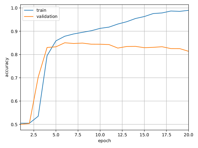
Train and validation accuracy for a transformer-like network using lambda layers instead of attention layers. Each lambda layer uses a convolution for the positional lambda.
The validation accuracy first rises sharply during the first few epochs before reaching a plateau and then slowly decreasing. This second phase, due to overfitting, can be easily corrected by reducing the number of epochs, so it will not be an issue in actual applications. (Notice that it happens while the train accuracy is already significantly higher than the validation accuracy; a simple algorithm can thus easily stop training before the overfitting starts to be an issue.)
More importantly, the validation accuracy reached just before that is a bit above 84%. So, although we have eliminated the quadratic scaling in memory required to run the network, we achieve the same accuracy after the same number of epochs! The big difference is that this model is much more scalable: while the problem we have tested it on is relatively simple (simple enough that the input data can be efficiently batched on a typical desktop GPU despite the quadratic memory requirement of standard transformers), this network can be extended to much more intensive ones for which usual transformers would be impractical or require an unrealistic amount of memory.
For this reason, and since the optical Fourier transform, with its O(1) scaling, is the most efficient way to perform large convolutions, we believe that the future of transformers lies in optical computing. We hope to release more results soon, so stay tuned!
class LambdaConvolutionLayer2D(torch.nn.Module):

    def __init__(self, context_size: Tuple[int, int], in_channels: int, input_size: Tuple[int, int], k_size: int):
        assert (input_size[0] == input_size[1])
        assert (k_size >= 1)
        super(LambdaConvolutionLayer2D, self).__init__()
        self.input_size: Tuple[int, int] = input_size
        self.filter_size: Tuple[int, int] = context_size
        self.in_channels: int = in_channels
        self.k_size: int = k_size
        self.wk: Parameter = Parameter(torch.Tensor(self.in_channels, self.k_size))
        self.wv: Parameter = Parameter(torch.Tensor(self.in_channels, self.in_channels))
        self.wq: Parameter = Parameter(torch.Tensor(self.in_channels, self.k_size))
        self.positional_embedding_filter: Parameter = Parameter(
            torch.Tensor(self.filter_size[0], self.filter_size[1], self.k_size))
        self.softmax: torch.nn.Softmax = torch.nn.Softmax(dim=1)
        self.reset_parameters()

    def reset_parameters(self) -> None:
        torch.nn.init.uniform_(self.wk, -0.5, 0.5)
        torch.nn.init.uniform_(self.wv, -0.5, 0.5)
        torch.nn.init.uniform_(self.wq, -0.5, 0.5)
        torch.nn.init.uniform_(self.positional_embedding_filter, -0.5, 0.5)

    def forward(self, x) -> torch.Tensor:
        batch_size: int = x.shape[0]
        x_rearranged: torch.Tensor = x.permute(0, 3, 1, 2).reshape(batch_size, -1, self.in_channels)

        # query generation: x * wq -> Q (input_size * k_size)
        Q: torch.Tensor = self.to_queries(batch_size, x_rearranged)

        # context summary: x * wk -> K (input_size * k_size)
        K: torch.Tensor = self.to_keys(batch_size, x_rearranged)

        # value generation: x * wv -> V (channels * channels)
        V: torch.Tensor = self.to_values(batch_size, x_rearranged)

        # Lambda^C: K^T * V -> Lc (k_size * channels) : Content summary
        Lc: torch.Tensor = self.to_lc(K, V)

        # Lambda^P : Positional summary
        Lp: torch.Tensor = self.to_lp(batch_size, V)

        # Lambda attention
        return self.to_attention(batch_size, Lc, Lp, Q).permute(0, 3, 1, 2)

    def to_attention(self, batch_size: int, lc: torch.Tensor, lp: torch.Tensor, q: torch.Tensor) -> torch.Tensor:
        lambda_sum: torch.Tensor = lp + lc.view(
            lc.shape[0], 1, 1, lc.shape[1], lc.shape[2]
        ).repeat(1, self.input_size[0], self.input_size[1], 1, 1)
        flattened_ls: torch.Tensor = lambda_sum.view(batch_size, -1, lambda_sum.shape[3], lambda_sum.shape[4])
        reshaped_ls: torch.Tensor = flattened_ls.view(-1, flattened_ls.shape[2], flattened_ls.shape[3]).transpose(1, 2)
        return torch.bmm(
            reshaped_ls, q.view(reshaped_ls.shape[0], -1, 1)
        ).view(batch_size, self.input_size[0], self.input_size[1], self.in_channels)

    def to_lp(self, batch_size: int, v: torch.Tensor) -> torch.Tensor:
        # slow code for explanation
        # Lp = torch.zeros(batch_size, self.input_size[0], self.input_size[1], self.k_size, self.in_channels)
        # for k in range(self.k_size):
        #     for d in range(self.in_channels):
        #         _v = v[:, :, d].reshape(batch_size, self.input_size[0], self.input_size[1])
        #         _r = self.positional_embedding_filter[:, :, k]
        #         r_conv_v = F.conv2d(_v.view(batch_size, 1, self.input_size[0], self.input_size[1]),
        #                             _r.view(1, 1, self.filter_size[0], self.filter_size[1]),
        #                             padding=(int(self.filter_size[0] / 2), int(self.filter_size[1] / 2)))
        #         Lp[:, :, :, k, d] = r_conv_v.view(batch_size, self.input_size[0], self.input_size[1])

        # fast code
        v_conv: torch.Tensor = v.permute(0, 2, 1).view(
            batch_size, self.in_channels, self.input_size[0], self.input_size[1])
        r_conv: torch.Tensor = self.positional_embedding_filter.permute(2, 0, 1).repeat(self.in_channels, 1, 1)
        r_conv: torch.Tensor = r_conv.view(r_conv.shape[0], 1, r_conv.shape[1], r_conv.shape[2])
        lp: torch.Tensor = F.conv2d(v_conv, r_conv,
                                    padding=(int(self.filter_size[0] / 2), int(self.filter_size[1] / 2)),
                                    groups=self.in_channels)
        lp = lp.reshape(lp.shape[0], self.in_channels, self.k_size, lp.shape[2], lp.shape[3])
        return lp.permute(0, 3, 4, 2, 1)

    @staticmethod
    def to_lc(k: torch.Tensor, v: torch.Tensor) -> torch.Tensor:
        return torch.bmm(torch.transpose(k, 1, 2), v)

    def to_values(self, batch_size: int, x: torch.Tensor) -> torch.Tensor:
        return torch.bmm(x, self.wv.view(self.in_channels, self.in_channels).repeat(batch_size, 1, 1))

    def to_keys(self, batch_size: int, x: torch.Tensor) -> torch.Tensor:
        return self.softmax(
            torch.bmm(x, self.wk.view(1, self.in_channels, self.k_size).repeat(batch_size, 1, 1)))

    def to_queries(self, batch_size: int, x: torch.Tensor) -> torch.Tensor:
        return torch.bmm(x, self.wq.view(1, self.in_channels, self.k_size).repeat(batch_size, 1, 1))
Appendix: PyTorch code for the full Transformer network
Here we show the code for the classification transformer used in this study, drawing inspiration from from Peter Bloem’s GitHub repository.
# a transformer block with
#    * a self-attention layer,
#    * a normalization layer,
#    * a 2-layer perceptron applied to each vector with n*k neurons,
#    * a normalization layer,
# and residual connections between each of them
class TransformerBlock(nn.Module):

    def __init__(self, k, h=8, n=4):

        super().__init__()

        # attention layer
        self.attention = SelfAttention(k, h=h)

        # normalization layers
        self.norm1 = nn.LayerNorm(k)
        self.norm2 = nn.LayerNorm(k)

        # 2-layer perceptron with ReLU activation function
        self.perceptron = nn.Sequential(
            nn.Linear(k, n*k),
            nn.ReLU(),
            nn.Linear(n*k, k))

    def forward(self, x):
        y1 = self.attention(x)
        x = self.norm1(y1 + x)
        y2 = self.perceptron(x)
        return self.norm2(y2 + x)


# a classification transformer class
class CTransformer(nn.Module):

    def __init__(self, k, h, depth, seq_length, num_tokens, num_classes):

        super().__init__()

        # number of tokens
        self.num_tokens = num_tokens
        # token embedding
        self.token_emb = nn.Embedding(num_tokens, k)
        # position embedding
        self.pos_emb = nn.Embedding(num_tokens, k)

        # transformer blocks
        self.tblocks = nn.Sequential(*(TransformerBlock(k,h) for i in range(depth)))

        # map the output to class probabilities
        self.toprobs = nn.Linear(k, num_classes)

    def forward(self, x):
        '''
        Argument: a tensor x of size (b,t).
        Return: a tensor of size (b, num_class).
        '''

        # generate the token embeddings
        tokens = self.token_emb(x)
        b, t, k = tokens.size()

        # generate the position embeddings
        positions = self.pos_emb(torch.arange(t))[None,:,:].expand(b, t, k)

        x = self.tblocks(tokens + positions)
        x = self.toprobs(x.mean(dim=1))

        # apply the log_softmax activation function and return the result
        return F.log_softmax(x, dim=1)
¹ A variant of the transformer architecture, the Reformer, was proposed in early 2020 to reduce the memory requirement.
² The name DALL·E is a portmanteau word made of the last name of Spanish surrealist painter Salvador Dali and the character WALL·E from the eponymous animation movie by Pixar Animation Studios.
³ This ensures that all the trainable parameters for this layer are in the convolution functions.
News
© 2024 All rights reserved Optalysys Ltd
Subscribe
Sign up with your email address to receive news and updates from Optalysys.