
There are many reasons to be excited by FHE. The ability to perform computations on encrypted data is a game changer for many fields. Using FHE, users can have encrypted data processed by third parties. Processing is carried out entirely on encrypted data, yielding encrypted results.
Thus, a user can have their data processed by, say, a proprietary AI model owned by a medical company, without needing to share their data or compromise their privacy. In the event that the medial company experienced a data breach, no user information would be retrievable. It would all be encrypted.
Although this technology already exists, FHE requires a lot of compute power and can be prohibitively slow, limiting real work use cases. However, at Optalysys, we are currently building optical compute hardware that can accelerate real-world FHE workloads by over two orders of magnitude. We thus see our optical technology as the key to unlocking the huge potential of FHE.
We’ve already covered how we can merge Zama’s Concrete and Concrete-Boolean libraries with our technology, and used this combined system to carry out a range of tasks in encrypted space. We’ve also been transitioning from applications which are interesting (performing Conway’s Game of Life in encrypted space) through to applications which are useful.
Practical FHE
It’s well established that FHE is going to be revolutionary for the way that data can be handled, managed and analysed, which in turn is going to open up a vast new market in providing encrypted data services. However, to fully realise the commercial value, FHE has to be accessible to a far broader developer base than it currently is.
So to tie FHE together with familiar software development tasks, in this article we’ll be taking things to another level. We’ll demonstrate how we can securely implement a powerful data analysis tool and apply it to the test case of evaluating encrypted medical data. We’ll be leveraging the power of Zama’s Concrete library. This library has made it easier than ever to start applying powerful FHE techniques.
We consider the situation where a medical company has created a logistic regression AI model to predict the whether a patient has a disease based on their medical record. The patient would like to know if they have a disease, but do not want to expose their data to any security risks incurred by transmitting their data. We will therefore use FHE to allow the model to work with encrypted data.
The two diagrams below explain why FHE is necessary for such a system to be secure:

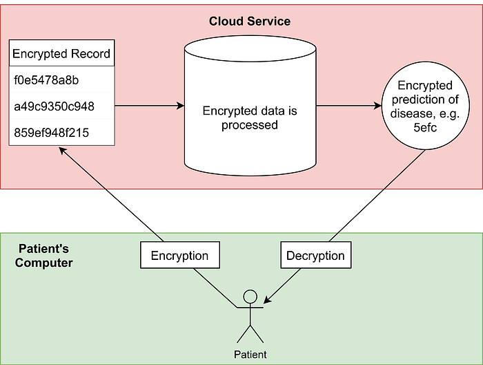
Leveraging FHE will allow this to take place; the user will receive a prediction of whether they have a disease, without their medical record being exposed to the third party, or any adversaries on the way.
Before discussing the FHE implementation, we will first introduce logistic regression and build a basic model.
What is logistic regression?
Logistic regression is a supervised learning technique to classify data. A logistic regression model is trained by optimising coefficients that are applied to a feature vector as a linear combination. Probabilistic predictions can be obtained by passing the output of the linear combination through a logistic function.
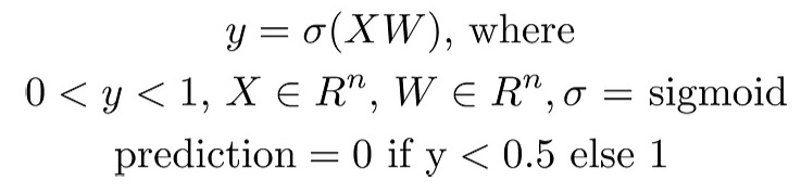
More formally, a scalar prediction y in the range (0, 1) is obtained by applying a logistic function (e.g. sigmoid) to a scalar value v, which is the output of dot product between a feature vector X and a learned weight vector W.
The prediction y can be interpreted as the probability of the input vector corresponding to one of two classes. A bias or intercept term can be added explicitly, or encoded via an additional weight and concatenating a 1 onto the feature vector.
Logistic regression is essentially linear regression, but instead of predicting a continuous output variable, it predicts a binary classification probability by applying a logistic function to the output.
Thus if we threshold the model output at 0.5, we can use it directly as a binary classifier. In this article, we are not interested in the output probability, only the class. As such we can omit the sigmoid function, instead thresholding the output of the linear model at 0.
Logistic Regression in Python
We can create and optimise a logistic regression model in Python using the NumPy and Scikit-learn packages. We will use these packages for the dataset, pre-processing, model generation, optimisation and evaluation.
Training the model
The following code snippet demonstrates how we can create a logistic regression model on Scikit-learn’s breast cancer dataset:
from sklearn.datasets import load_breast_cancer
from sklearn.linear_model import LinearRegression, LogisticRegression
from sklearn.preprocessing import normalize
import numpy as np

# load the breast cancer dataset
d = load_breast_cancer()

# normalise the features such that they lie in the range [0, 1]
x, y = normalize(d['data']), d['target']

# train the model
regressor = LogisticRegression().fit(x, y)

# predict with the model on the dataset
model_predictions = regressor.predict(x)

# check the accuracy of the model
print(regressor.score(x, y))

When we run this code, we find out that the accuracy of the model is 81%.
Visualising the model’s predictions
By plotting the data, we can visualise the decision boundary of the model. As we have a 9-dimensional feature vector, its hard to visualise, so we will plot the data in 2 dimensions, taking only the two features with the largest absolute coefficients in our model and plotting these on the x and y axes.
Points on the plot represent individual data samples, with their associated class label represented using colour. Below is a plot showing the output of our model’s predictions vs. the ground truth for our dataset. Positive predictions are shown in orange, negative blue.
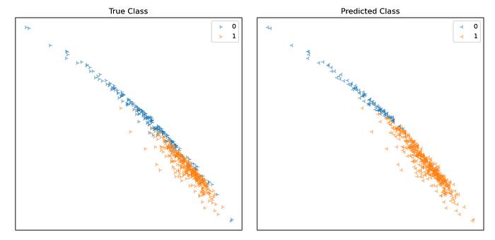
From the plots, we can see that many samples are being classified correctly. There seems to be a linear decision boundary that cuts the data fairly well, though some are being classified incorrectly.
Understanding the model and data dimensionality
The following code will tell us more about the dataset and the model’s parameters:
np.set_printoptions(precision=2, suppress=True)

# check the dimensionality of the data
print(x.shape)

# check the model weights and bias terms
print(regressor.coef_, regressor.intercept_)
Running this, we find out that the shape of the dataset, model weights and bias (the .coef_ and .intercept_ parameter respectively) are (to two d.p.):
Dataset shape: (569,30)
Weights: [[ 0.61 1.16 3.69 4.87 0.01 0. -0. -0. 0.01 0.01 0.01 0.1
0.04 -0.8 0. 0. 0. 0. 0. 0. 0.58 1.45 3.48 -4.55
0.01 -0. -0.01 -0. 0.02 0.01]]
Bias: [0.34]
Many of these values are very low, indicating that the associated features are contribute very little to the prediction. It is therefore likely that we can simplify this model, which we will do in the next section of the article.
For now, we will save the model weights and dataset to a csv file for use later in Concrete via Rust:
# saves a model and a dataset to file
# bias is interpreted as an additional feature with value 1
# for each dataset item, and a model weight == bias
def save_weights_and_data(weights, bias, data):
	bias = bias.reshape((1,1))
	weights = np.concatenate((bias, weights), axis=1).flatten()
	data = np.concatenate((np.ones((data.shape[0], 1)), data), axis=1).transpose().flatten()
	np.savetxt("data.csv", data, fmt="%1.6f")
	np.savetxt("weights.csv", weights, fmt="%1.6f")

 save_weights_and_data(weights, bias, data)


This function will save each element to a new line. We store a vector of weights that comprise the model, and a flattened 2D array for the dataset.
Simplifying the model
Simplifying the model is an important step because we can remove redundant computation, hopefully without affecting the quality of the prediction.
There are many sophisticated approaches to feature selection, however we will opt for a simple one for brevity’s sake. Let’s try to simplify the model by choosing an arbitrary threshold for feature weights, discarding those weights that are below the threshold based on the assumption that low weights do not contribute much to the model’s predictions.
# reduce dimensionality of weights and data, based on weighting threshold
def get_reduced_coef_and_data(model, x, threshold):
	features = np.where(np.abs(regressor.coef_[0]) >= threshold)[0]
	return model.coef_[:, features], x[:, features]

weights, data = get_reduced_coef_and_data(regressor, x, threshold=0.5)
Setting the threshold to 0.5 reduces the dimensionality of the weights and items in the dataset from 30 to 9, reducing the model size and required computation by a factor >3. Lets now test the model to see it still predicts effectively.
First we will define a function to predict directly from the weight, bias and data NumPy arrays:
# convert a real value to class prediction using sign
def to_binary_prediction(x):
	return (x > 0).astype(int)

# generate predictions from np arrays
def predict_from_matrices(data, weights, bias):
	pred = np.matmul(data, weights.transpose()) + bias
	return to_binary_prediction(pred[:,0])

We will now define a function to compare the similarity of model outputs:
def binary_prediction_similarity(pa, pb):
	return 1 - np.mean(np.abs(pa - pb))
This function will return a value in the range 0 and 1 denoting the similarity of the two binary prediction arrays. For two arrays that are the same we will get a value of 1, and for two arrays that are completely different, we would get a value of 0.
We can now test the similarity of the full model that uses 30 features, vs. the streamlined model with only 9:
full_model_predictions = regressor.predict(x)

bias = regressor.intercept_
weights, data = get_reduced_coef_and_data(regressor, x, threshold=0.5)
reduced_model_prediction = predict_from_matrices(data, weights, bias)

print(binary_prediction_similarity(full_model_predictions, reduced_model_prediction))
The output of the code is 1.0. In short, the model with 9 features is predicting exactly the same as the model with 30, so we have significantly reduced the complexity of the model without compromising any performance.
We can now re-run the code that saves the new weights and dataset with fewer features, such that our .csv files contain the simplified model and data.
Implementing the model in Concrete
We will use the Concrete library to perform homomorphic inference using the trained model on encrypted data. The Concrete library significantly simplifies implementing this kind of thing. In the next sections we will focus primarily on practical use of the library, leaving out some low-level implementation details for brevity.
Loading Data
First we will load our data and model weights into vectors in Rust:
// imports for file reading
use std::fs::File;
use std::io::{BufRead, BufReader, Error, ErrorKind, Read};

// helper function to print elements of a vector
fn print_f64_vector(v: &Vec::<f64>){
    for &element in v { print!("{}, ", element); }
    println!("");
}

// function to read the csv files
fn read<R: Read>(io: R) -> Result<Vec<f64>, Error> {
    let br = BufReader::new(io);
    br.lines()
        .map(|line| line.and_then(|v| v.parse().map_err(|e| Error::new(ErrorKind::InvalidData, e))))
        .collect()
}

fn main() -> Result<(), Box<dyn std::error::Error>> {
    // read the data: you will have to change the path!
    let plaintext_data = read(File::open("/home/ed/py/linreg/weights.csv")?)?;
    let cipher_data_input = read(File::open("/home/ed/py/linreg/data.csv")?)?;

    // make sure we have read the values correctly
    print_f64_vector(&plaintext_data);
    print_f64_vector(&cipher_data_input);

    Ok(())
}
Concrete implementation of Logistic Regression
The next step is to implement the FHE-powered logistic regression model in Rust with Concrete. We’ll do this using the following stages:
- Create an encoder using Concrete that will be used to when encrypting and decrypting the patient’s medical data.
- Create two secret keys using Concrete, used to encrypt and decypt the data.
- Create a bootstrap key using the secret keys. This is what allows the encrypted data to be operated on. The bootstrap key is shared with the medical company in our example use case. This remains secure because the bootstrap key does not allow data to be decrypted into plaintext (see our previous article for a more detailed description of what bootstrapping is and why it works).
- Create some custom error types, useful if there are problems when we run novel operations.
- Create two structs for matrices containing plaintext and encrypted ciphertext data. We will use these to store the model weights and patient data respectively.
- Write a matrix multiply function that can operate on plaintext and encrypted matrices.
- Combine the above elements to make the encrypted logistic regression model.
With all the above pieces, we will be able to: encrypt patient data; store it in matrix form; store plaintext model data in matrix form; and multiply the two matrices homomorphically to obtain encrypted predictions. We will then use the patient’s secret key to decrypt the model predictions and assess if the homomorphic model works as expected.
1–3. Defining the encoding and the encryption keys
First we need some extra imports from the Concrete library:
# concrete imports
pub use concrete::{ Encoder, LWESecretKey, RLWESecretKey, LWEBSK, LWEKSK, LWE, LWE128_1024, RLWE128_1024_1,CryptoAPIError };

Now we can define the input encoder, secret keys and the bootstrap key in the main function:
// define an encoder for the input with parameters:
//    range of inputs (-2, 2)
//    bits of precision = 6
//    bits of padding = 7
let encoder_input = Encoder::new(-2., 2., 6, 7)?;

// secret keys with parameters:
//    bits of security = 128
//    polynomial size = 1024
let sk_rlwe = RLWESecretKey::new(&RLWE128_1024_1);
let sk_in = LWESecretKey::new(&LWE128_1024);

// bootstrap key with parameters:
//    log base = 6
//    levels = 8
let bsk = LWEBSK::new(&sk_in, &sk_rlwe, 6, 8);
The parameters used above took a bit of fine tuning, for more information on how these parameters work please look at the Concrete documentation.
4–5. Defining the matrix structs (and custom errors)
As we are creating new operations and operands, we first define some error types that we will use later:
/// A custom error for FHE operations
#[derive(Debug, Clone)]
pub struct FHEError { message: String }
impl FHEError {
    pub fn new(message: String) -> FHEError { FHEError { message } }
}

impl std::fmt::Display for FHEError {
    fn fmt(&self, f: &mut std::fmt::Formatter) -> std::fmt::Result {
        write!(f, "FHEError: {}", self.message)
    }
}

impl std::error::Error for FHEError {}
impl std::convert::From<CryptoAPIError> for FHEError {
    fn from (err: CryptoAPIError) -> Self {
        FHEError::new(format!("CryptoAPIError: {:}", err))
    }
}

/// a matrix operation error
#[derive(Debug, Clone)]
struct MatOpError { message: String }
impl std::fmt::Display for MatOpError {
    fn fmt(&self, f: &mut std::fmt::Formatter) -> std::fmt::Result {
        write!(f, "{}", self.message)
    }
}

impl std::error::Error for MatOpError {}
impl MatOpError {
    fn new(message: String) -> MatOpError { MatOpError { message } }
}

Now we must define the ciphertext matrix struct, then implement a new method which will allow us to create matrices of ciphertexts. The data containing the elements of the ciphertext matrix is stored in a vector of type LWE:
/// a matrix of LWE ciphers
pub struct CipherMatrix {
    pub dimensions: (usize, usize),
    pub data: Vec<LWE>
}

impl CipherMatrix {

    pub fn new(data: Vec<LWE>, dimensions: (usize, usize))
        -> Result<CipherMatrix, FHEError>
    {
        // check that the data has the right number of elements
        if data.len() != dimensions.0 * dimensions.1 {
            return Err(FHEError::new(format!(
                "The dimensions are ({}, {}), so the data must have {} elements, but has {}",
                dimensions.0, dimensions.1, dimensions.0 * dimensions.1, data.len()
            )))
        }
        Ok(CipherMatrix { dimensions, data })
    }
}
We similarly define a plaintext matrix containing 64-bit floats:
/// a matrix of plaintext values
pub struct PlaintextMatrix {
    pub dimensions: (usize, usize),
    pub data: Vec<f64>
}

impl PlaintextMatrix {

    pub fn new(data: Vec<f64>, dimensions: (usize, usize))
        -> Result<PlaintextMatrix, FHEError>
    {
        // check that the data has the right number of elements
        if data.len() != dimensions.0 * dimensions.1 {
            return Err(FHEError::new(format!(
                "The dimensions are ({}, {}), so the data must have {} elements, but has {}",
                dimensions.0, dimensions.1, dimensions.0 * dimensions.1, data.len()
            )))
        }
        Ok(PlaintextMatrix { dimensions, data })
    }
}
6. Writing the matrix multiply function
Matrix multiplication is defined in the usual way. We first check the dimensions of the two matrices to make sure they can be multiplied, then we create a result vector of the right size. We accumulate each output term in this vector, and return a newly created ciphertext matrix containing the data.
fn safe_mul_constant_with_padding(cipher: &LWE, constant: f64, max_pt_val: f64, bits_to_consume: usize)
    -> Result<LWE, Box<dyn std::error::Error>>
{
    if constant != 0. {
        Ok(
            cipher.mul_constant_with_padding(
                constant, max_pt_val, bits_to_consume
            )?
        )
    }
    else{
        Ok(
            cipher.add_centered(
                &cipher.opposite()?
            )?.mul_constant_with_padding(
                1.0, max_pt_val, bits_to_consume
            )?
        )
    }
}

pub fn mat_mul_pc(m1: &PlaintextMatrix, m2: &CipherMatrix, bsk: &LWEBSK, max_pt_val: f64, bits_to_consume: usize)
    -> Result<CipherMatrix, Box<dyn std::error::Error>>
{
    check_dims_pc(m1, m2)?;
    let mut ans_vector = Vec::<LWE>::with_capacity(m1.dimensions.0 * m2.dimensions.1);
    for ay in 0..m1.dimensions.0{
        for ax in 0..m2.dimensions.1{
            println!("{}, {}", ay, ax);
            for val in 0..m1.dimensions.1{
                if val == 0{
                    ans_vector.push(
                        safe_mul_constant_with_padding(
                            &m2.data[ax],
                            m1.data[ay*m1.dimensions.1],
                            max_pt_val,
                            bits_to_consume
                        )?
                    );
                }
                else{
                    ans_vector[ax + (m2.dimensions.1 * ay)].add_centered_inplace(
                        &m2.data[ax + (val*m2.dimensions.1)].mul_constant_with_padding(
                            m1.data[(ay*m1.dimensions.1) + val], max_pt_val, bits_to_consume
                        )?
                    )?;
                }
                ans_vector[ax + (m2.dimensions.1 * ay)].bootstrap(bsk)?;
            }
        }
    }
    Ok(
        CipherMatrix::new(ans_vector, (m1.dimensions.0, m2.dimensions.1))?
    )
}
This function uses a couple of functions from the Concrete library, namely add_centered_inplace and mul_constant_with_padding. We wont go into the details of how these work, but at a high level they are simply addition and multiplication functions. add_centered_inplace adds two ciphertexts together, and mul_constant_with_padding multiplies a ciphertext by a plaintext constant, returning a new ciphertext.
We define a function called safe_mul_constant_with_padding that removes some issues when using mult_constant_with_padding on a constant that is zero. The technical details of this are a bit much for the scope of this article, but what the function is doing can be understood as follows:
Aim: calculate (C*0), where C is a ciphertext
Workflow: return (C+(C*-1)) * 1.0
This function ensures that the output is correct, and that it has the right format and encoding such that later operations are compatible with the cipher.
7. Putting it all together
We now have all the required elements to run the logistic regression model on some encrypted data. Here’s how we do it:
fn main() -> Result<(), Box<dyn std::error::Error>> {
    // dimensions of the matrices
    let plaintext_matrix_dimensions: (usize, usize) = (1,10);       // model weights
    let cipher_matrix_dimensions: (usize, usize) = (10,569);        // dataset

    // read weights and data from files
    let plaintext_data = read(File::open("/home/ed/py/linreg/weights.csv")?)?;
    let cipher_data_input = read(File::open("/home/ed/py/linreg/data.csv")?)?;

    // encoders: min val, max val, bits, bits of padding
    let encoder_input = Encoder::new(-2., 2., 6, 7)?;

    // secret keys: 128 bits of security, polnomial size of 1024
    let sk_rlwe = RLWESecretKey::new(&RLWE128_1024_1);
    let sk_in = LWESecretKey::new(&LWE128_1024);

    //bootstrapping key: log base of 6, 8 levels
    let bsk = LWEBSK::new(&sk_in, &sk_rlwe, 6, 8);

    // encrypt each message
    let cipher_data: Result<Vec<LWE>, _> = cipher_data_input.into_iter().map(|m|
        LWE::encode_encrypt(&sk_in, m, &encoder_input)).collect();

    // build a matrix with the cipher and plaintext
    let plaintext_mat = PlaintextMatrix::new(plaintext_data, plaintext_matrix_dimensions)?;
    let ciphertext_mat = CipherMatrix::new(cipher_data?, cipher_matrix_dimensions)?;

    // multiply the matrices
    let mat_mul_result_cipher = mat_mul_pc(&plaintext_mat, &ciphertext_mat, &bsk, 5., 6)?;

    // decrypt the result
    let mat_mul_result_plaintext = decrypt_vector(&mat_mul_result_cipher.data, &sk_in)?;

    // print the model output
    print_f64_vector(&mat_mul_result_plaintext);

    Ok(())
}
The output of the above code is a list of numbers, the sign of these numbers indicates the class of the prediction, negative sign, negative prediction and vice versa:
-1.1276431618729381, -0.26699129985757963, …0.6429439321792962
Results
After a bit of post processing of the data in Python to retrieve the class predictions, we can plot the predictions of the model. We will plot them in the same way as before: taking the two dimensions of the input features with the highest associated coefficients in the model. We will compare the output predictions of the plaintext model with the model that works on encrypted inputs.
Encrypted model using FHE:

Plaintext model:
The two plots look identical. This is good news as it suggests that the model that uses encrypted data seems to be working as well as the original plaintext model.
However, to confirm this, we ran the binary_prediction_similarity function described earlier to compare the two models’ predictions. We found a prediction similarity of 0.995 or 99.5%. This is a result of the models disagreeing on 3 single data points out of 569, which may be as a result of precision limitations in the chosen parameters for Concrete.
This means that the model converted to run on encrypted inputs works almost identically to its plaintext counterpart. We were happy with the balance of runtime and accuracy, although it is possible to achieve even greater accuracy.
If, for instance, we used a higher bit precision in our encoder, perhaps with a larger polynomial size, it is likely that we could remove any discrepancy between the two models, but there would be an associated runtime cost.
Conclusion
We have shown how to create a logistic regression model in Python, how to interpret the results, and how to convert such a model to work with Zama’s Concrete FHE library. Using FHE, we have shown that we can create a logistic regression model that works entirely on encrypted data. Using fairly performant parameter choices, able to run inference in a reasonable length of time, we were able to run the model on encrypted data without sacrificing acccuracy.
Our model is able to predict disease from an encrypted medical record, without the data ever being exposed. Patients can encrypt their own medical record, send it a to a medical company for processing, and receive an encrypted result.
At Optalysys we know that technology like this is the key to solving many risks and concerns surrounding data processing. We foresee a future that leverages a combination of FHE algorithms with optical hardware acceleration, removing many user privacy concerns, and allowing models to be built on data shared without risk.